Matrix Multiplication with AlphaEvolve

Introduction

Matrix multiplication is a foundational operation in computer science, powering a wide range of applications – from deep learning model training to 3D graphics transformations. Modern neural networks spend most of their compute time multiplying weight matrices with activations, and 3D rendering pipelines apply successive matrix transforms to rotate or project scenes. Any improvement in matrix multiplication efficiency can thus have far-reaching impact.
Volker Strassen’s 1969 algorithm was the first to break the $O(n^3)$ time barrier, using a clever divide-and-conquer method to multiply matrices in $O(n^{\log_2 7}) \approx O(n^{2.8074})$ operations [wiki]. This remained the best general method for square matrix multiplication for decades, as faster algorithms existed only for huge matrices or special cases. In June 2025, a DeepMind research team introduced AlphaEvolve, an AI-driven system that discovered a faster way to multiply two $4\times 4$ matrices using only 48 scalar multiplications – the first improvement in 56 years over Strassen’s 49-multiplication scheme over a noncommutative ring. This breakthrough, documented in the [AlphaEvolve arXiv paper], in theory opens a new chapter in matrix algorithms, demonstrating that even long-standing bounds can be beaten by novel techniques.

Overall Goal of the Project

You will investigate these algorithmic advancements. You will implement Strassen’s classical fast matrix multiplication and the newly published AlphaEvolve $4\times 4$ algorithm in C++, then benchmark their performance and analyze their trade-offs. By reimplementing these algorithms and testing them on various setups, you will gain a deep understanding of why Strassen’s method stood unchallenged for 56 years and what enabled AlphaEvolve’s improvement.

0. Standard $2\times 2$ Matrix Multiplication Algorithm

Given two $2 \times 2$ block matrices $A$ and $B$, we want to compute $C = AB$. The standard algorithm computes each element as a dot product:

Copy LaTeX $$\begin{pmatrix} {\color{green} A_{11}} & {\color{green} A_{12}} \\ {\color{green} A_{21}} & {\color{green} A_{22}} \end{pmatrix} \times \begin{pmatrix} {\color{orange} B_{11}} & {\color{orange} B_{12}} \\ {\color{orange} B_{21}} & {\color{orange} B_{22}} \end{pmatrix} = \begin{pmatrix} {\color{teal} C_{11}} & {\color{teal} C_{12}} \\ {\color{teal} C_{21}} & {\color{teal} C_{22}} \end{pmatrix}, \quad {\color{teal} C_{ij}} = \sum\limits_{k=1}^2 {\color{green} A_{ik}} \cdot {\color{orange} B_{kj}}$$

This gives us the following partial products:

$$\begin{align} m_1 &= {\color{green} A_{11}} \cdot {\color{orange} B_{11}} \\ m_2 &= {\color{green} A_{12}} \cdot {\color{orange} B_{21}} \\ m_3 &= {\color{green} A_{11}} \cdot {\color{orange} B_{12}} \\ m_4 &= {\color{green} A_{12}} \cdot {\color{orange} B_{22}} \\ m_5 &= {\color{green} A_{21}} \cdot {\color{orange} B_{11}} \\ m_6 &= {\color{green} A_{22}} \cdot {\color{orange} B_{21}} \\ m_7 &= {\color{green} A_{21}} \cdot {\color{orange} B_{12}} \\ m_8 &= {\color{green} A_{22}} \cdot {\color{orange} B_{22}} \end{align}$$

And the final result elements are computed as:

$$\begin{align} {\color{teal} C_{11}} &= m_1 + m_2 \\ {\color{teal} C_{12}} &= m_3 + m_4 \\ {\color{teal} C_{21}} &= m_5 + m_6 \\ {\color{teal} C_{22}} &= m_7 + m_8 \end{align}$$

The naive approach requires 8 matrix multiplications.

1. Strassen’s $2\times 2$ Matrix Multiplication Algorithm

In 1969, Volker Strassen astonished the computer science community by showing that matrix multiplication could be performed with fewer multiplications than the conventional $n^3$ method. Strassen’s algorithm multiplies two $2\times 2$ block matrices using only 7 submatrix multiplications (instead of 8), recombining them with addition and subtraction to produce the final product.

$$\begin{align} m_1 &= ({\color{green}A_{11}} + {\color{green}A_{22}})\cdot({\color{orange}B_{11}} + {\color{orange}B_{22}}) \\ m_2 &= ({\color{green}A_{21}} + {\color{green}A_{22}})\cdot{\color{orange}B_{11}} \\ m_3 &= {\color{green}A_{11}}\cdot({\color{orange}B_{12}} - {\color{orange}B_{22}}) \\ m_4 &= {\color{green}A_{22}}\cdot({\color{orange}B_{21}} - {\color{orange}B_{11}}) \\ m_5 &= ({\color{green}A_{11}} + {\color{green}A_{12}})\cdot{\color{orange}B_{22}} \\ m_6 &= ({\color{green}A_{21}} - {\color{green}A_{11}})\cdot({\color{orange}B_{11}} + {\color{orange}B_{12}}) \\ m_7 &= ({\color{green}A_{12}} - {\color{green}A_{22}})\cdot({\color{orange}B_{21}} + {\color{orange}B_{22}}) \end{align}$$

These products are then recombined to form the result blocks:

$$\begin{align} {\color{teal} C_{11}} &= m_1 + m_4 - m_5 + m_7 \\ {\color{teal} C_{12}} &= m_3 + m_5 \\ {\color{teal} C_{21}} &= m_2 + m_4 \\ {\color{teal} C_{22}} &= m_1 - m_2 + m_3 + m_6 \end{align}$$

How Strassen Arrived at Discovery

1. A Bilinear Approach to the Problem

Strassen didn't start by trying to improve matrix multiplication directly. He was working on a more general problem - the rank of bilinear forms in algebraic complexity theory. The key insight was that matrix multiplication can be represented as a bilinear map:

$$f: \mathbb{C}^{n \times n} \times \mathbb{C}^{n \times n} \to \mathbb{C}^{n \times n}$$

2. Tensor Rank and Decomposition

Strassen understood that the complexity of matrix multiplication is related to the tensor rank of the corresponding tensor. For $2 \times 2$ matrices, the naive algorithm gives a rank of 8, but Strassen sought a decomposition with lower rank. The breakthrough came when Strassen realized that operations could be redistributed. Instead of computing each element of the result directly, he devised intermediate quantities $m_1, m_2, \ldots, m_7$ that simultaneously capture information about multiple elements.

3. Algebraic Manipulations

Strassen used classical algebraic tricks:

Linear combinations: $(A + B)(C + D) = AC + AD + BC + BD$
Compensating terms: if you need $AC$ but computed $(A + B)(C + D)$, subtract the unwanted $AD$, $BC$, $BD$
Operation grouping: multiple result elements can be obtained from the same intermediate products

Let's look at the logic behind the first one of Strassen's products:

$$ m_1 = ({\color{green}A_{11}} + {\color{green}A_{22}}) \cdot ({\color{orange}B_{11}} + {\color{orange}B_{22}}) \\ $$

This product simultaneously "captures" information for the diagonal elements of the result $\color{teal} C_{11}$ and $\color{teal} C_{22}$. Strassen realized that such grouping allows for product operation savings.

4. Systematic Search

He didn't guess the formulas randomly. He:

Wrote down a system of equations for all elements $\color{teal} C_{ij}$
Searched for ways to express them through a minimal number of products
Used algebraic identities to minimize the number of multiplications

Why Was This So Difficult?

Before Strassen, everyone believed that $n^3$ was the natural lower bound
Trade-offs: Strassen's algorithm requires more additions and memory - one had to understand that this was an acceptable price
The algorithm's power only manifests when recursively applied to large matrices

Recursively applying this idea yields an asymptotic complexity of $O(n^{\log_2 7}) \approx O(n^{2.8074})$, beating the standard $O(n^3)$ runtime. This was profound and opened an entire field of research - searching for optimal tensor decompositions for various matrix sizes, which remains an active area of investigation to this day.

2. Winograd’s $4\times 4$ Matrix Multiplication Algorithm

For $4\times 4$ Matrix Multiplication Strassen's decomposition gives $7\times 7 = 49$ multiplications. In fact, [Winograd's 1968 paper] on computing inner products faster could be applied to $4\times 4$ matrix multiplication to get a formula using only 48 multiplications.

Winograd's Key Insight

Winograd's breakthrough came from recognizing the algebraic identity:

$$a_1b_1 + a_2b_2 = (a_1 + b_2)(a_2 + b_1) - a_1a_2 - b_1b_2$$

It changes two multiplications of ab's into one multiplication of ab's and two multiplications involving only a's or only b's. The latter multiplications can be pre-computed and saved when calculating all the innerproducts in a matrix multiplication:

$$\begin{align} i=1..4, &\text{ 8 multiplications:} \\ &p_i = -A_{i1} \times A_{i2} - A_{i3} \times A_{i4} \\ \text{another} &\text{ 8 multiplications:} \\ &q_i = -B_{1i} \times B_{2i} - B_{3i} \times B_{4i} \\ i=1..4,\ &j=1..4\ \text{ finally } 4 \times 4 \times 2 = 32 \text{ multiplications:} \\ &C_{ij} = p_i + q_j \\ &+ (A_{i1} + B_{2j}) \times (A_{i2} + B_{1j}) + \\ &+ (A_{i3} + B_{4j}) \times (A_{i4} + B_{3j}) \end{align}$$

In total, we got $8 + 8 + 32 = 48$ multiplications. When looking at this result from DeepMind in 2025, you might wonder - if Winograd achieved a formula with 48 multiplications back in 1968, what makes the DeepMind result significant? The key difference lies in generality. Winograd's method only works when the matrix entries commute with each other (i.e., $ab = ba$). In contrast, tensor decomposition formulas like DeepMind's work even over noncommutative rings. This may seem like an obscure distinction, but it becomes highly relevant when dealing with matrices of matrices - a common case in practice. Since matrices themselves don't commute, Winograd's approach can't be used recursively on larger matrices. Tensor decomposition formulas, however, can be applied recursively, making them more powerful for general matrix multiplication.

3. What the hell are these tensor decompositions?

Let's return to the Strassen's $2 \times 2$ matrix multiplication algorithm, and rewrite formulas using tensor decomposition. So we still want to calculate the $2 \times 2$ matrix product, but we can represent it as a 3D $4 \times 4 \times 4$ tensor:

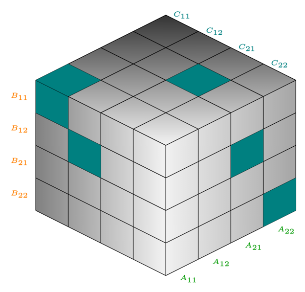
Copy LaTeX $$\begin{pmatrix} {\color{green} A_{11}} & {\color{green} A_{12}} \\ {\color{green} A_{21}} & {\color{green} A_{22}} \end{pmatrix} \times \begin{pmatrix} {\color{orange} B_{11}} & {\color{orange} B_{12}} \\ {\color{orange} B_{21}} & {\color{orange} B_{22}} \end{pmatrix} = \begin{pmatrix} {\color{teal} C_{11}} & {\color{teal} C_{12}} \\ {\color{teal} C_{21}} & {\color{teal} C_{22}} \end{pmatrix}, \quad {\color{teal} C_{ij}} = \sum\limits_{k=1}^2 {\color{green} A_{ik}} \cdot {\color{orange} B_{kj}}$$

Tensor representation of $2 \times 2$ matrix multiplication. For example ${\color{teal} C_{22}} = {\color{green} A_{21}} \cdot {\color{orange} B_{12}} + {\color{green} A_{22}} \cdot {\color{orange} B_{22}}$

The tensor $T_{ijk} = 1$ when element $A_{ik}$ multiplied by $B_{kj}$ contributes to $C_{ij}$, following the standard matrix multiplication rule:

$$C_{ij} = \sum_{k} A_{ik} \cdot B_{kj} \cdot T_{ijk}$$

Intermediate Products	Result Combinations
$$\begin{align} m_1 &= ({\color{green}A_{11}} + {\color{green}A_{22}})\cdot({\color{orange}B_{11}} + {\color{orange}B_{22}}) \\ m_2 &= ({\color{green}A_{21}} + {\color{green}A_{22}})\cdot{\color{orange}B_{11}} \\ m_3 &= {\color{green}A_{11}}\cdot({\color{orange}B_{12}} - {\color{orange}B_{22}}) \\ m_4 &= {\color{green}A_{22}}\cdot({\color{orange}B_{21}} - {\color{orange}B_{11}}) \\ m_5 &= ({\color{green}A_{11}} + {\color{green}A_{12}})\cdot{\color{orange}B_{22}} \\ m_6 &= ({\color{green}A_{21}} - {\color{green}A_{11}})\cdot({\color{orange}B_{11}} + {\color{orange}B_{12}}) \\ m_7 &= ({\color{green}A_{12}} - {\color{green}A_{22}})\cdot({\color{orange}B_{21}} + {\color{orange}B_{22}}) \end{align}$$	$$\begin{align} {\color{teal} C_{11}} &= m_1 + m_4 - m_5 + m_7 \\ {\color{teal} C_{12}} &= m_3 + m_5 \\ {\color{teal} C_{21}} &= m_2 + m_4 \\ {\color{teal} C_{22}} &= m_1 - m_2 + m_3 + m_6 \end{align}$$

Intermediate Products

Result Combinations

So Strassen's algorithm in rank-1 tensors decomposition looks like this:

One-rank tensor representation of two terms $m_1$ and $m_2$. Watch carefully for signs in formulas for elements of $\color{teal} C$.

$$T = \sum\limits_{i=1}^7 u_i \otimes v_i \otimes w_i$$

Tensor Game

The tensor game is a game where one player takes turns to find some tensor decomposition. Consider the game is played on matrices $A$ and $B$, and the goal is to find a tensor $T$ corresponding to the matrix multiplication.

Starting state $S_0 = T$
Your move: choose one-rank tensor $(u_t, v_t, w_t)$
New state: $S_{t+1} \leftarrow S_t - u_t \otimes v_t \otimes w_t $
Repeat until $S_{t+1} = 0$, reward is -1 per step

AlphaTensor Ingredients to Win the Game

1. Special Architecture

One neural network to predict value (how close we are to final move) and policy (one-rank tensor $(u_t, v_t, w_t)$), as in AlphaZero
Projections of the original 3D tensor to three 2D features' matrices
Sequence of attention operations, each over a set of features belonging to one tensor slice

2. Synthetic Demonstrations

There is asymmetry: going from original tensor $T$ to one-rank decomposition is hard and going back is very simple.

3. Target Diversification

Express the target in several equivalent ways via change of basis (this is clearly just data augmentation :).

4. Train a Generalist Agent

Consider all the dimensions of the tensor simultaneously, limiting the maximum only. Actually zero-padding works perfectly for this purpose.

AlphaTensor Limitations

We have to use only a finite set of coefficients before multipliers: $F = \{-2, -1, 0, 1, 2\}$. So this method cannot guarantee optimality. It is not a general method for any searched space, only for tensor decompositions.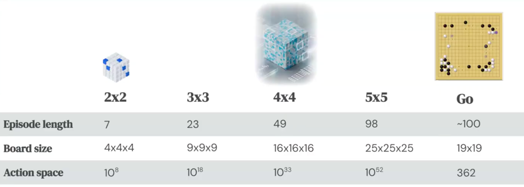

The search difficulty is incredible! Source: Alex Novikov talk

4. Next Step: AlphaEvolve

An evolutionary coding agent to optimize and discover algorithms.

Key ingredients:

Creativity of LLMs
Rigorous and automated Evaluation
Diversity of Evolution

FunSearch	AlphaEvolve
evolve 1 function	evolve entire module
up to S-size LLMs	benefits from latest LLMs
1e6 LLM samples needed	1e3 LLM samples can suffice
evaluation must be fast (<= 20 mins)	evaluation can be slow & parallelized
feedback only from code execution	can additionally leverage LLM feedback
no additional context provided	long context provided
evolve Python	evolve any evaluable (string) content
evolution: optimize 1 metric	evolution: optimize multiple metrics

AlphaEvolve search process visualization, source

5. Results for $4 \times 4$ matrix multiplication

Algorithm	Multiplications	Additions
Naïve	64	48
Strassen, 1969	49	318 (~132 with optimizations)
Winograd, 1968	48	128
AlphaEvolve, 2025	48	1264
Rosowski, 2019	46	133

6. Algorithm Engineering Task for Students

Your task is to implement a benchmark in C++ to measure the performance of the listed algorithms, similar to the table Sub-cubic algorithms that should also include both time and memory usage metrics. Compare different matrix sizes, types (e.g. random, symmetric), and hardware setups to analyze the trade-offs between algorithmic complexity, memory overhead, numerical stability and parallelism.

Part 1: Implementation

Check different matrix sizes and different matrix types (e.g., random, symmetric, etc.). Aim for a clean, well-structured implementation from scratch – do not use any built-in matrix multiplication libraries or Strassen routines. While coding, consider the memory overhead (allocate auxiliary matrices for intermediate computations as needed) and keep track of the number of scalar multiplications and additions being performed (you will use this in analysis).

Part 2: Benchmarking the Algorithms

With all the algorithms implemented, the next step is to empirically evaluate their performance. Theoretical operation counts tell us that the AlphaEvolve algorithm uses fewer multiplications than Strassen’s (and far fewer than the $64$ multiplications of the naive $4\times 4$ multiply), but actual runtime depends on many factors: constant factors from additions, memory access patterns, parallelism, etc. By benchmarking, we can observe how these algorithms behave in practice on real hardware. Additionally, we want to see how they scale beyond the base $4\times 4$ case – e.g., can we leverage the 48-multiplication method to multiply larger matrices more quickly via a recursive blocking approach? This experiment will shed light on whether AlphaEvolve’s theoretical advantage translates into real speedups and under what conditions.

Design and run a comprehensive set of benchmarks comparing algorithms. You should consider the following scenarios:

Matrix sizes and blocking: Test not just $4\times 4$ matrices, but larger sizes as well. For example, try $8\times 8$, $16\times 16$, $64\times 64$, up to sizes like $256\times 256$ or $512\times 512$ (if feasible).
Real vs Complex data: Benchmark both algorithms on matrices with real numbers and with complex numbers. Compare the runtime of multiplying real-valued matrices using each algorithm. Then do the same for complex-valued matrices (where a naive algorithm would itself require more operations, since multiplying complex numbers takes multiple real multiplications). This will illustrate how each algorithm benefits different data types.
Hardware setups: Run your benchmarks on different hardware environments if possible. At minimum, test on a CPU. If you have access to a GPU or a multi-core processor, attempt to run the algorithms there as well (Note: you may need to port your code or use a library to utilize GPU acceleration). For instance, you might compare a single-threaded CPU execution to a multi-threaded one, or CPU vs GPU, to see how well each algorithm parallelizes. If implementing your own code on GPU is too complex, you can still compare your CPU implementations to a highly-optimized GPU matrix multiply (e.g. BLAS or CuBLAS library) for reference. The goal is to observe how hardware influences the efficacy of these algorithms.

For each test scenario, record metrics such as: the wall-clock running time (in milliseconds or seconds) of each algorithm, and possibly the number of arithmetic operations executed (you can instrument your code to count scalar multiplications and additions). Use sufficiently many trials and/or large enough problem sizes to get stable timing results (to mitigate noise). Organize your benchmark results clearly – for example, you might tabulate the timings for various sizes, or plot the performance curves if you have many data points.

Part 3: Analyzing Algorithmic Trade-offs

In the final step, you will analyze and interpret the results of your implementations and experiments. High-level algorithmic improvements do not automatically guarantee practical superiority; this project is an opportunity to understand why. By reflecting on the data and the nature of each algorithm, you will consolidate your understanding of where each approach shines or struggles. This analysis connects theory with practice: you’ll consider factors like arithmetic counts (multiplications vs additions), memory usage, and numerical precision, explaining in your own words how these factors influence performance on real hardware.

Write a concise report or summary interpreting the comparative performance algorithms, based on your benchmarking results and implementation experience. In your analysis, address the following points:

Operation counts: Summarize the theoretical number of multiplications and additions each algorithm uses. Discuss how this reduction in multiplications affected your measured performance. Did fewer multiplications generally translate to faster runtime? Explain how extra additions might diminish the benefit of saving multiplications, especially on modern CPUs/GPUs where addition is relatively cheap but not free. If you counted operations in your code, report the observed counts and confirm they match the expected formula.
Memory overhead and access patterns: Compare the memory requirements of the two algorithms. Strassen’s algorithm, for instance, needs auxiliary matrices to store intermediate sums (in an optimized implementation, Strassen can be done with a small constant factor more memory, but naive multiplication can be done in-place with minimal extra space). AlphaEvolve’s algorithm likely required even more scratch space to hold many intermediate linear combinations. Describe any memory allocation and copying that your implementations had to do. How might this extra memory usage impact performance (consider cache misses and data movement)? If you ran on large matrices, did you notice any performance issues related to memory (e.g., higher memory usage causing slowdowns)?
Numerical stability: Reflect on the numerical stability of each approach. Both Strassen and the AlphaEvolve algorithm use subtractions which can lead to cancellation and rounding error. Strassen’s algorithm is known to be slightly less stable than the naive algorithm (because it subtracts large intermediate values). AlphaEvolve’s algorithm might be even more delicate, given it uses complex multipliers and many operations – for example, coefficients like $1/2$ and imaginary units could amplify rounding issues in floating-point arithmetic. If possible, report on any experiments you did to test stability: e.g. multiplying matrices with condition number extremes or random data to see if results diverge or lose accuracy compared to naive multiplication. Even if you did not explicitly test this, discuss theoretically which algorithm you expect to introduce more numerical error and why.
Hardware and parallelism impact: Analyze how each algorithm fared across different hardware setups. For instance, if you tested on a GPU or multi-core CPU, was either algorithm able to take advantage of parallelism effectively? Discuss the fact that naive matrix multiplication is highly optimized on modern hardware (using SIMD instructions, cache blocking, etc.), whereas your implementations of Strassen/AlphaEvolve might not have benefited from such low-level optimizations. It’s possible that on a GPU, the straightforward $O(n^3)$ algorithm (as used in libraries) vastly outperformed your recursive algorithms for all tested sizes, because those algorithms introduce irregular memory access and cannot use the GPU’s matrix-multiply units as efficiently. Comment on any such observations: for example, “On CPU, Strassen began to outperform the naive method for $n > 128$, but on GPU the naive BLAS routine was faster than both Strassen and AlphaEvolve even at $n=512$,” etc. Relate this to the trade-off between algorithmic complexity and constant factors: the cross-over point where an asymptotically faster algorithm wins may be very large, and highly optimized conventional algorithms (especially on specialized hardware) can dominate for practical matrix sizes.
Overall takeaways: Conclude with a summary of what you learned. For example, you might note that while AlphaEvolve’s algorithm is a stunning theoretical advancement, its practical benefit is subtle. The reduction of one multiplication (about a 2% cut in multiplication count for $4\times 4$) is very likely outweighed by the quadrupling of addition operations and more complex data flow, which is why Strassen’s algorithm stood unbeaten for so long – any better algorithm inherently had to be much more complex. You should also mention how this exercise gave insight into the difficulty of improving matrix multiplication: even a small $4\times 4$ case required AI assistance and led to an algorithm with many caveats. Finally, consider the broader implication: as matrix sizes grow, the slight exponent improvement (from $\approx 2.8074$ to $\approx 2.7925$ for exponent in the recursive sense) might become noticeable, but only if implementations can efficiently manage the overhead. Will future computers benefit from this 48-multiplication algorithm? Or will practical factors (like memory and stability) limit its use? Your analysis should demonstrate a nuanced understanding of these questions, backed by the evidence you gathered in your benchmarks.