Machine Learning with Python
Lecture 13. Intro to neural networks and backpropagation
Alex Avdiushenko
November 14, 2023
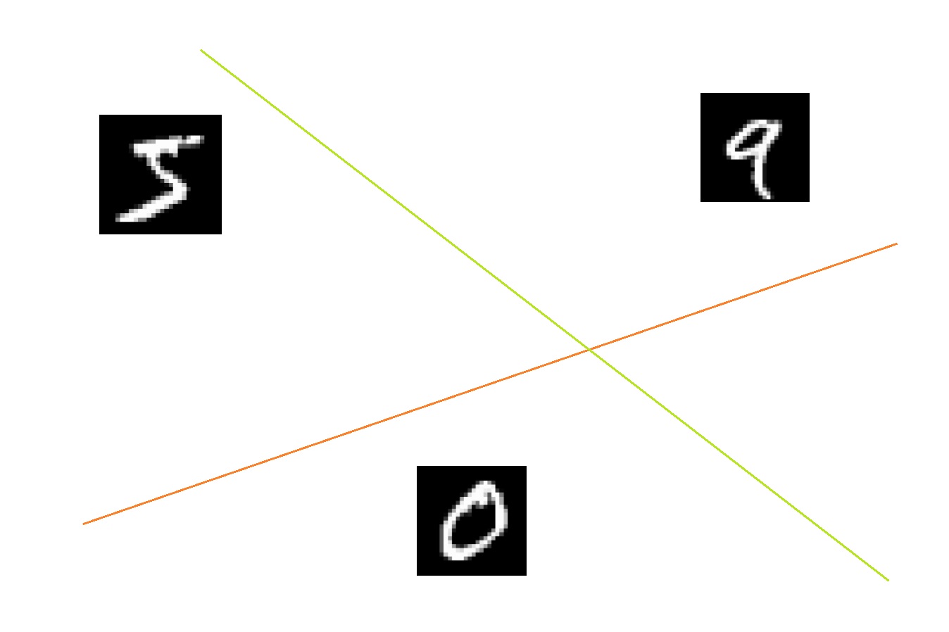
Images
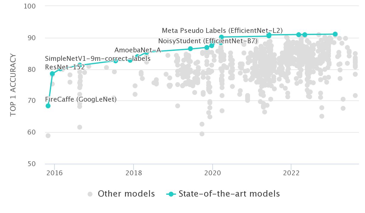
 25% $\to$ 3.5% errors versus 5% in humans
|
Text

|
Voice

|
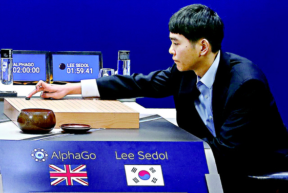
Go, 2016
|
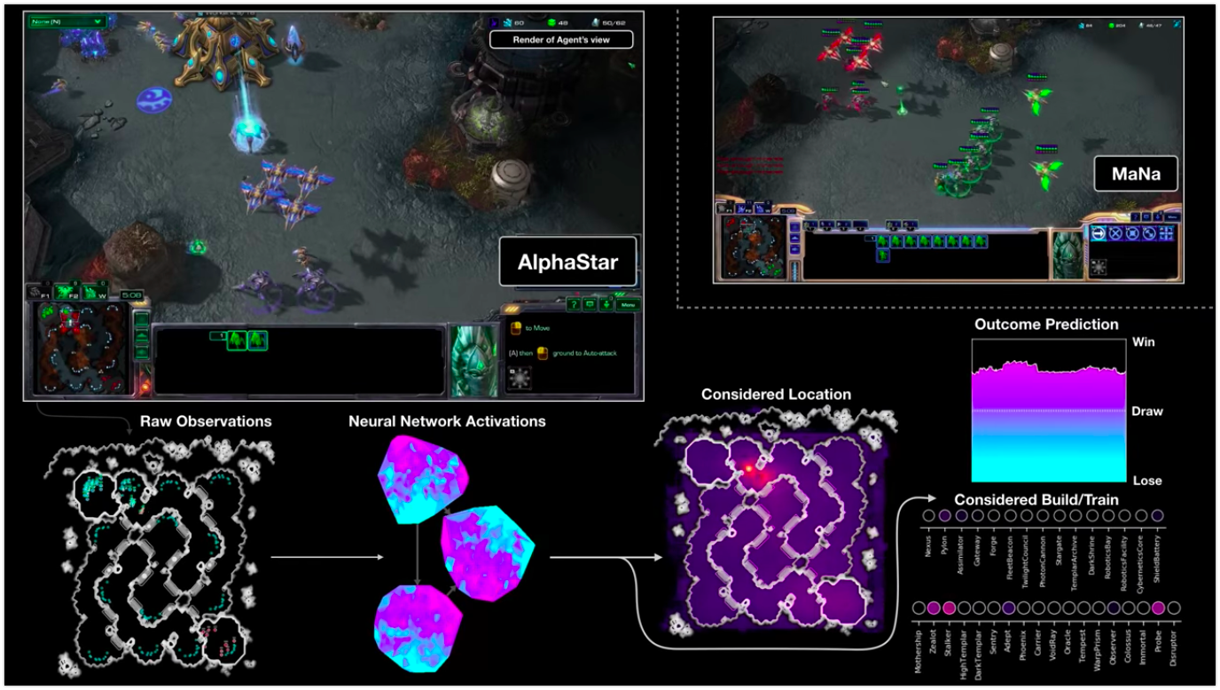
StarCraft, 2019
|
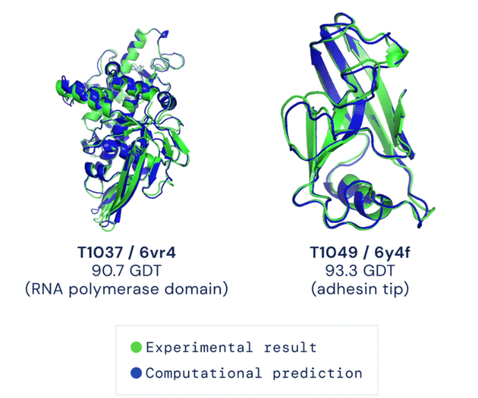
Protein structure, 2020
|
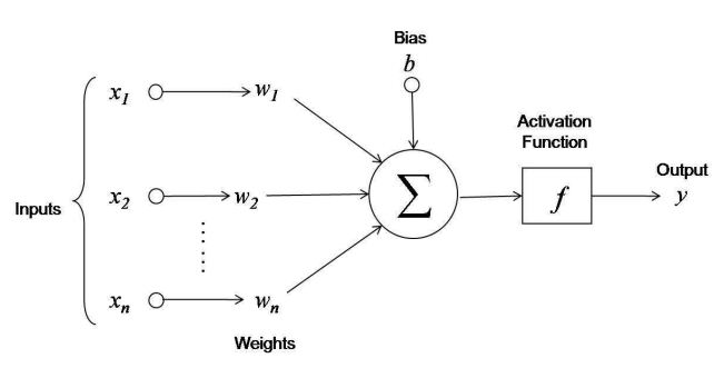
Linear Model (Reminder)
$f_j: X \to \mathbb{R}$ — numerical features
$$a(x, w) = f(\left< w, x\right>) = f\left(\sum\limits_{j=1}^n w_j f_j(x)+b \right)$$where $w_1, \dots, w_n \in \mathbb{R}$ — feature weights, $b$ — bias
$f(z)$ — activation function, for example, $\text{sign}(z),\ \frac{1}{1+e^{-z}},\ (z)_+$
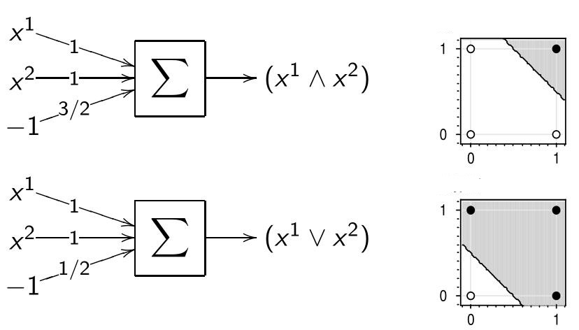
Neural Implementation of Logical Functions
The functions AND, OR, NOT from binary variables $x^1$ and $x^2$:
$x^1 \wedge x^2 = [x^1 + x^2 - \frac{3}{2} > 0]$
$x^1 \vee x^2 = [x^1 + x^2 - \frac{1}{2} > 0]$
$\neg x^1 = [-x^1 + \frac{1}{2} > 0]$
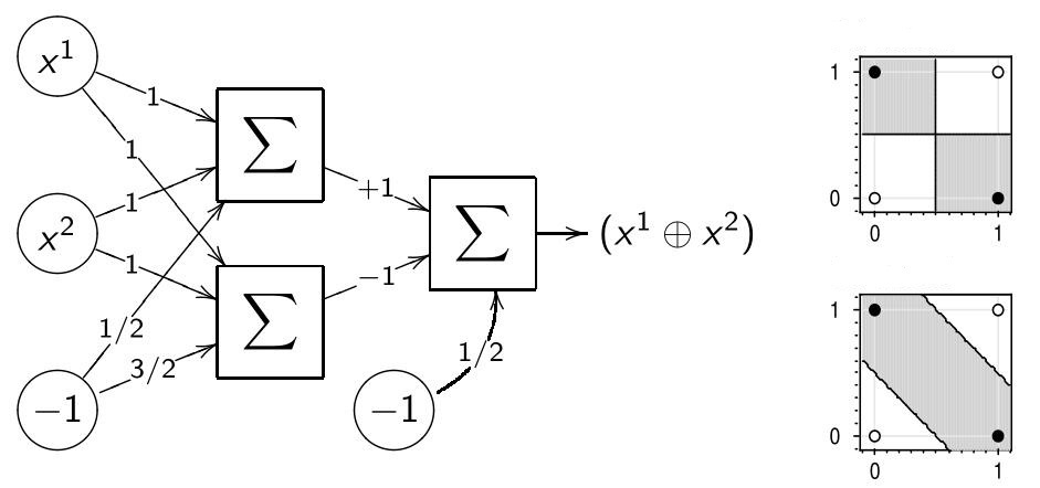
Logical XOR Function (Exclusive OR)
Function $$x^1 \bigoplus x^2 = [x^1 \neq x^2]$$ is not implementable by a single neuron. There are two ways to implement:
- Adding nonlinear feature: $$x^1 \bigoplus x^2 = [x^1 + x^2 - {\color{orange}2x^1 x^2} - \frac12 > 0]$$
- Network (two-layer superposition) of AND, OR, NOT functions: $$x^1 \bigoplus x^2 = [(x^1 \vee x^2) - (x^1 \wedge x^2) - \frac12 > 0]$$
Expressive Power of Neural Network
- A two-layer network in $\{0, 1\}^n$ can implement any arbitrary Boolean function
- A two-layer network in $\mathbb{R}^n$ can separate any arbitrary convex polyhedron
- A three-layer network in $\mathbb{R}^n$ can separate any polyhedral region (may not be convex or connected)
- Using linear operations and one nonlinear activation function $\sigma$, any continuous function can be approximated with any desired accuracy
- For some special classes of deep neural networks, it has been proven that they have exponentially higher expressive power than shallow networks.
V. Khrulkov, A. Novikov, I. Oseledets. Expressive power of recurrent neural networks, Feb , ICLR 2018
Expressive Power of Neural Network
Function $\sigma(z)$ — sigmoid, if $\lim\limits_{z \to -\infty} \sigma(z) = 0$ and $\lim\limits_{z \to +\infty} \sigma(z) = 1$
Cybenko's Theorem
If $\sigma(z)$ is a continuous sigmoid, then for any continuous function $f(x)$ on $[0,1]^n$, there exist such parameter values $w_h \in \mathbb{R}^n, b \in \mathbb{R}, \alpha_h \in \mathbb{R}$ that a single-layer network $$a(x) = \sigma\left(\sum\limits_{h=1}^H \alpha_h \left< x, w_h\right> + b\right)$$ uniformly approximates $f(x)$ with any desired accuracy $\varepsilon$: $|a(x) - f(x)| < \varepsilon$, for all $x \in [0, 1]^n$
G. Cybenko. Approximation by Superpositions of a Sigmoidal Function. Mathematics of Control, Signals, and Systems (MCSS) 2 (4): 303-314 (Dec 1, 1989)
Linear Classifier
Prediction $y_{pred} = x \cdot W + b$
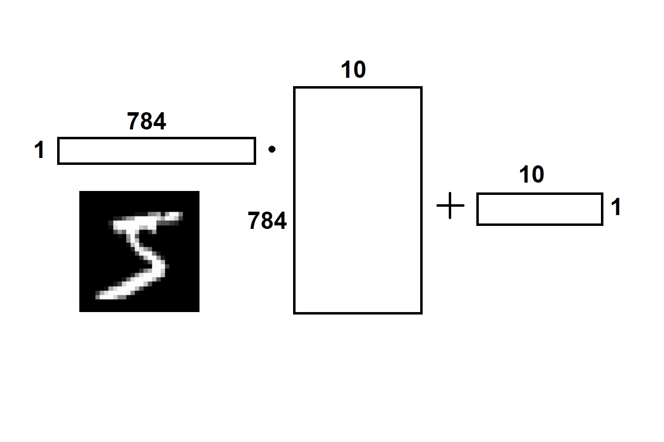
$\quad x\quad\quad\cdot\quad W\quad\quad+\quad b\quad$
Ten Separating Planes
In our example, the space is 784-dimensional: $\mathbb{R}^{784}$
If $y_{true, i} \in \mathbb{R}$ (that is, the task of linear regression), then to minimize the sum of the squares of differences (least squares method), the answer is calculated analytically by the formula:
$$\hat{W} = (X^TX)^{-1}X^T y_{true}$$In general, it is solved numerically by minimizing the loss function. Most often by gradient descent.
Softmax — for Classification
We transform our responses of the linear model into class probabilities:
$$ p(c=0| x) = \frac{e^{y_0}}{e^{y_0}+e^{y_1}+\dots+e^{y_n}} = \frac{e^{y_0}}{\sum\limits_i e^{y_i}} \\ p(c=1| x) = \frac{e^{y_1}}{e^{y_0}+e^{y_1}+\dots+e^{y_n}} = \frac{e^{y_1}}{\sum\limits_i e^{y_i}} \\ \dots $$Principle of Maximum Likelihood (Reminder)
$$\arg\max\limits_w {P(Y|w, X)P(w)} {\color{orange}=} \arg\max\limits_w \prod\limits_{i=1}^\ell {P(y_i|w, x_i)P(w)} = \\ \arg\max\limits_w \sum\limits_{i=1}^\ell \log P(y_i|w, x_i) + \log P(w)$$Minimization of Loss Function
$$L(w) = \sum\limits_{i=1}^\ell {\mathcal{L}(y_i, x_i, w)} = -\ln P(y_i|w, x_i) \to \min\limits_w$$This is cross-entropy loss for the case $y_i \in \{0, 1\}$. In our case:
$$ L(W, b) = - \sum\limits_j \ln \frac{e^{(x_jW + b)_{y_j}}}{\sum\limits_i e^{(x_jW + b)_{i}}}$$We find the minimum of the function by stochastic gradient descent:
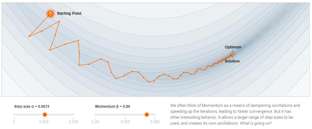
$$ W^{k+1} = W^{k} - \eta \frac{\partial L}{\partial W} \\ b^{k+1} = b^{k} - \eta \frac{\partial L}{\partial b} \quad\quad$$Mini-batch Training
We reduce the variance of the gradient.
Input: sample $X^\ell$, learning rate $\eta$, forgetting rate $\lambda$
Output: weight vector $w \equiv (w_{jh}, w_{hm})$
- Initialize the weights
- Initialize the functional assessment $Q = \frac{1}{\ell} \sum\limits_{i=1}^\ell \mathcal{L}_i (w)$
Repeat:
- Select $M$ objects $x_i$ from $X^\ell$ at random
- Calculate the loss: $\varepsilon = \frac{1}{M} \sum\limits_{i=1}^M \mathcal{L}_i (w)$
- Take the gradient step: ${\color{orange}w = w - \eta \frac{1}{M} \sum\limits_{i=1}^M \nabla \mathcal{L}_i (w)}$
- Estimate the functional: $Q = \lambda \varepsilon + (1 - \lambda) Q$
Until the value of $Q$ and/or the weight $w$ converges
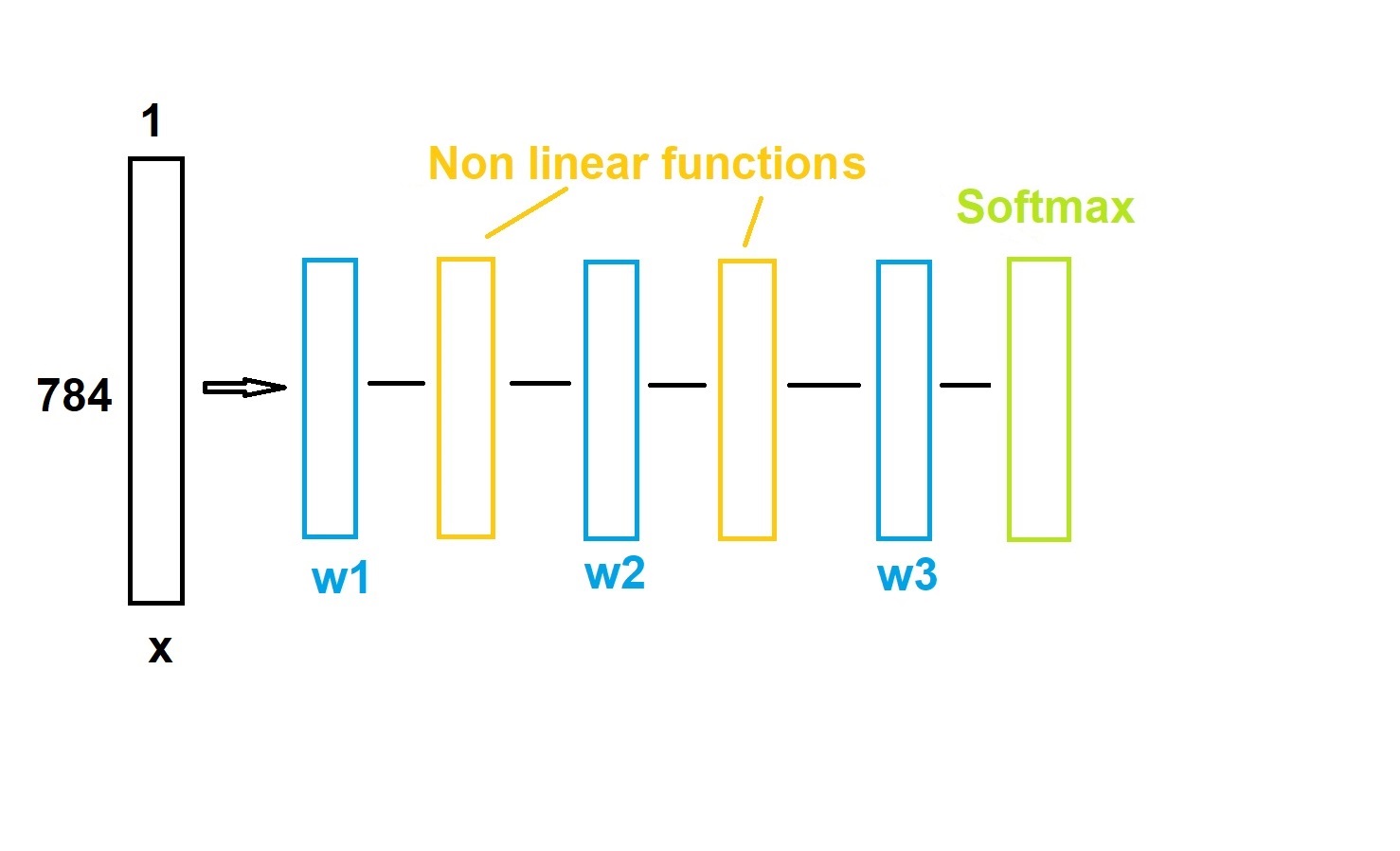
Neural network
Summary
- Neuron = Linear classification or regression
- Neural network = Superposition of neurons with a non-linear activation function
- BackPropagation = Fast differentiation of superpositions. Allows training of networks of virtually any configuration
- Methods to improve convergence and quality:
- Training on mini-subsets (mini-batch)
- Different activation functions
- Regularization