Machine Learning Intro

Machine Learning with Python

Lecture 5. Machine Learning Intro

Alex Avdiushenko
October 17, 2023

What is ML?

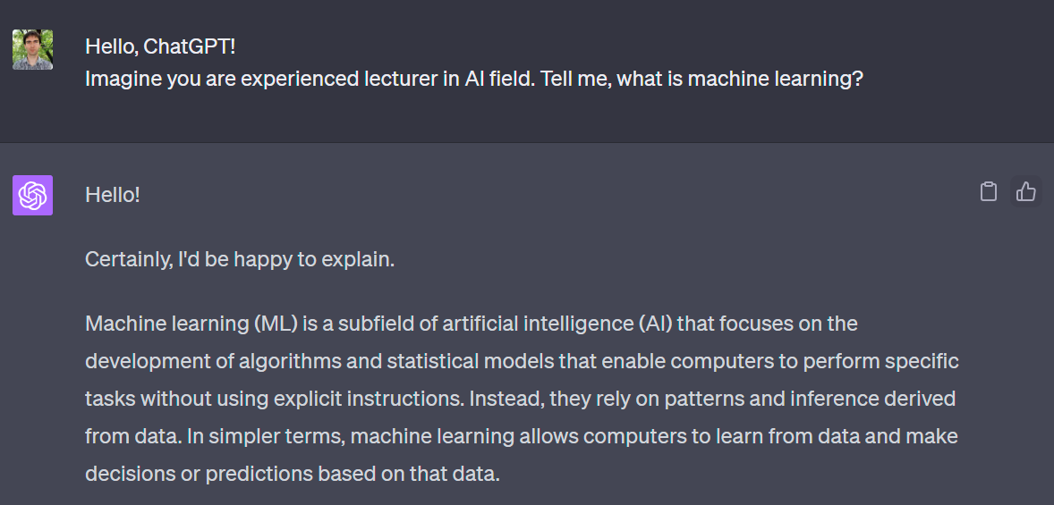
ML is built using the tools of mathematical statistics, numerical methods, mathematical analysis, optimization methods, probability theory, graph theory, and various techniques for working with data in digital form.

What is it?

\[\begin{cases} \frac{\partial \rho}{\partial t} + \frac{\partial(\rho u_{i})}{\partial x_{i}} = 0 \\ \\ \frac{\partial (\rho u_{i})}{\partial t} + \frac{\partial[\rho u_{i}u_{j}]}{\partial x_{j}} = -\frac{\partial p}{\partial x_{i}} + \frac{\partial \tau_{ij}}{\partial x_{j}} + \rho f_{i} \end{cases} \]

In machine learning, there is no pre-set model with equations...

Types of Machine Learning

Supervised Learning: The algorithm is provided with labeled training data, and the goal is to learn a general rule that maps inputs to outputs
Unsupervised Learning: The algorithm is provided with unlabeled data and must find the underlying structure in the data, like clustering or dimensionality reduction
Reinforcement Learning: The algorithm learns by interacting with an environment and receiving feedback in the form of rewards or penalties

Main notations

$X$ — set of objects
$Y$ — set of answers

$y: X \to Y$ — unknown dependence (target function)

The task is to find, based on the training sample $\{x_1,\dots,x_\ell\} = X_\ell \subset X$ with known answers $y_i=y(x_i)$,
an algorithm ${\color{orange}a}: X \to Y$,
which is a decision function that approximates $y$ over the entire set $X$.

The whole ML course is about this:

how objects $x_i$ are defined and what answers $y_i$ can be
in what sense ${\color{orange}a}$ approximates $y$
how to construct the function ${\color{orange}a}$

$f_j: X \to D_j$

The vector $(f_1(x), \dots, f_n(x))$ — feature description of the object $x$

Types of features:

$D_j = \{0, 1\}$ — binary
$\#|D_j| < \infty $ — categorical
$\#|D_j| < \infty, D_j$ ordered — ordinal
$D_j = \mathbb{R}$ — real (quantitative)

Data matrix (objects and features as rows and columns)

$F = ||f_j(x_i)||_{\ell\times n} = \left[ {\begin{array}{ccc} f_1(x_1) & \dots & f_n(x_1) \\ \vdots & \ddots & \vdots \\ f_1(x_\ell) & \dots & f_n(x_\ell) \end{array} } \right]$

Question 1: How to convert all features to binary?

Types of tasks

Classification

$Y = \{-1, +1\}$ — binary classification
$Y = \{1, \dots, M\}$ — multiclass classification
$Y = \{0, 1\}^M$ — multiclass with overlapping classes

Regression

$Y = \mathbb{R}$ or $Y = \mathbb{R}^m$

Ranking

$Y$ — finite ordered set

Predictive Model

A model (predictive model) — a parametric family of functions

$A = \{g(x, \theta) | \theta \in \Theta\}$,

where $g: X \times \Theta \to Y$ — a fixed function, $\Theta$ — a set of allowable values of parameter $\theta$

Example

Linear model with vector of parameters $\theta = (\theta_1, \dots, \theta_n), \Theta = \mathbb{R}^n$:

$g(x, \theta) = \sum\limits_{j=1}^n \theta_jf_j(x)$ — for regression and ranking, $Y = \mathbb{R}$

$g(x, \theta) = \mathrm{sign}\sum\limits_{j=1}^n \theta_jf_j(x)$ — for classification, $Y = \{-1, +1\}$

Example: Regression Task, Synthetic Data

$X = Y = \mathbb{R}$, $\ell = 50$ objects

$n = 3$ features: $\{1, x, x^2\}$ or $\{1, x, \sin x\}$

import matplotlib.pyplot as plt import numpy as np np.random.seed(0) l = 50 x = np.linspace(0, 30, num=l) Y = x + 4*np.sin(x) + 3*np.random.randn(l) X_1 = np.vstack([np.ones_like(x), x, x**2]).T X_2 = np.vstack([np.ones_like(x), x, np.sin(x)]).T print(X_1.shape, X_2.shape)

fig, ax = plt.subplots() ax.set_xlabel('x'), ax.set_ylabel('Y') ax.plot(x, Y, '.', label='train points') x_plot = np.linspace(0, 30, num=1000) ax.plot(x_plot, x_plot + 4*np.sin(x_plot), label='real') plt.legend(loc='best') fig # plt.show()

from sklearn.linear_model import LinearRegression reg_1 = LinearRegression(fit_intercept=False) reg_1.fit(X_1, Y) reg_2 = LinearRegression(fit_intercept=False) reg_2.fit(X_2, Y)

Question 2: What does an intercept mean?

fig, ax = plt.subplots() ax.set_xlabel('x'), ax.set_ylabel('Y') ax.plot(x, Y, '.', label='train points') x_plot = np.linspace(0, 30, num=1000) X_1 = np.vstack([np.ones_like(x_plot), x_plot, x_plot**2]).T X_2 = np.vstack([np.ones_like(x_plot), x_plot, np.sin(x_plot)]).T ax.plot(x_plot, reg_1.predict(X_1), label='{1, x, x^2}', linestyle='dashed') ax.plot(x_plot, reg_2.predict(X_2), label='{1, x, sin(x)}') plt.legend(loc='best') fig

Training Stage

The method $\mu$ constructs an algorithm $a = \mu(X_\ell, Y_\ell)$ from the sample $(X_\ell, Y_\ell) = (x_i, y_i)_{i=1}^\ell$

$\boxed{ \left[ {\begin{array}{ccc} f_1(x_1) & \dots & f_n(x_1) \\ \dots & \dots & \dots \\ f_1(x_\ell) & \dots & f_n(x_\ell) \end{array} } \right] \xrightarrow{y} \left[ {\begin{array}{c} y_1 \\ \dots \\ y_\ell \end{array} }\right] \thinspace} \xrightarrow{\mu} a$

Test Stage

The algorithm $a$ produces answers $a(x_i^\prime)$ for new objects $x_i^\prime$

Quality Functionals

$\mathcal{L}(a, x)$ — loss function. The error magnitude of the algorithm $a \in A$ on the object $x \in X$

Loss Functions for Classification Tasks:

$\mathcal{L}(a, x) = [a(x)\neq y(x)]$ — indicator of error
Cross entropy

Loss Functions for Regression Tasks:

$\mathcal{L}(a, x) = |a(x) - y(x)|$ — absolute error value
$\mathcal{L}(a, x) = (a(x) - y(x))^2$ — quadratic error

Empirical risk — functional quality of the algorithm $a$ on $X^\ell$:

$Q(a, X^\ell) = \frac{1}{\ell} \sum\limits_{i=1}^\ell \mathcal{L}(a, x_i)$

Reducing the Learning Task to an Optimization Task

Method of minimizing empirical risk

$\mu(X^\ell) = \arg\min\limits_{a \in A} Q(a, X^\ell)$

Example: least squares method ($Y = \mathbb{R}, \mathcal{L}$ is quadratic)

$\mu(X^\ell) = \arg\min\limits_{\theta} \sum\limits_{i=1}^{\ell} (g(x_i, \theta) - y_i)^2$

Generalization Ability Problem

Will we find the "law of nature" or will we overfit, i.e., adjust the function $g(x_i, \theta)$ to the given points?
Will $a = \mu(X^\ell)$ approximate the function $y$ over the entire $X$?
Will $Q(a, X^k)$ be small enough on new data — the test set $X^k = (x_i^\prime, y_i^\prime)_{i=1}^k$, $y_i^\prime = y(x_i)$?

Simple Example of Overfitting

Dependency $y(x) = \frac{1}{1+25x^2}$ on the interval $x \in \left[-2, 2\right]$

Feature description $x \to (1, x, x^2, \dots, x^n)$

Polynomial regression model:

$a(x, \theta) = \theta_0 + \theta_1 x + \dots + \theta_n x^n$ — a polynomial of degree $n$

Training using the least squares method:

$Q(\theta, X^\ell) = \sum\limits_{i=1}^\ell (\theta_0 + \theta_1 x_i + \dots + \theta_n x_i^n - y_i)^2 \to \min\limits_{\theta_0,\dots,\theta_n}$

Training sample: $X^\ell = \{x_i = 4\frac{i-1}{\ell-1} - 2 | i = 1, \dots, \ell \}$

Test sample: $X^k = \{x_i = 4\frac{i-0.5}{\ell-1} - 2 | i = 1, \dots, \ell-1 \}$

What happens to $Q(\theta, X^\ell)$ and $Q(\theta, X^k)$ as $n$ increases?

import numpy as np np.random.seed(0) l = 50 x = np.linspace(-2, 2, num=l) Y = 1 / (1 + 25*x**2) print(x.shape, Y.shape)

import matplotlib.pyplot as plt fig, ax = plt.subplots() ax.set_xlabel('x'), ax.set_ylabel('Y') ax.plot(x, Y, '.', label='train points') x_plot = np.linspace(-2, 2, num=1000) y_plot = 1 / (1 + 25*x_plot**2) ax.plot(x_plot, y_plot, label='real') plt.legend(loc='best') fig

from sklearn.linear_model import LinearRegression def X(x, n): res = [np.ones_like(x)] for i in range(1, n): res.append(x**i) return np.vstack(res).T print("X has been compiled.")

x_l = np.array([4*(i - 1)/(l - 1) - 2 for i in range(1, l + 1)]) x_k = np.array([4*(i - 0.5)/(l - 1) - 2 for i in range(1, l)]) lin_reg = LinearRegression(fit_intercept=False) train_score, test_score = [], [] ns = range(2, 40) for n in ns: X_l = X(x_l, n) Y_l = 1 / (1 + 25*x_l**2) X_k = X(x_k, n) Y_k = 1 / (1 + 25*x_k**2) lin_reg.fit(X_l, Y_l) train_score.append(np.mean((lin_reg.predict(X_l) - Y_l)**2)) test_score.append(np.mean((lin_reg.predict(X_k) - Y_k)**2)) print(n,end=', ') print()

import matplotlib.pyplot as plt_ fig_, ax_ = plt_.subplots() ax_.set_xlabel('n'), ax_.set_ylabel('log Q') ax_.set_xlim(0, len(ns) + 2) ax_.plot(np.log(train_score), 'bo-', label='train score') ax_.plot(np.log(test_score), 'go--', label='test score') plt_.legend(loc='best') # plt_.savefig('overfitting.png') print('OK!')

Question 3: Why we have such plots? How will the divergence point $n$ change depending on the size of the training sample $\ell$ and why?

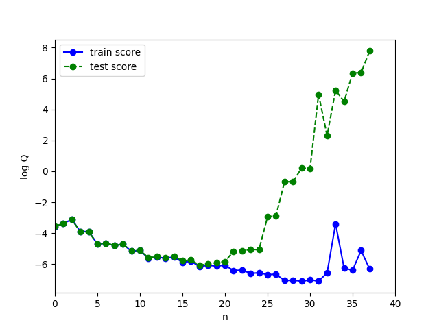
Overfitting — one of the main problems in machine learning

When test_score >> train_score

What causes overfitting?
- Excessive complexity of the parameter space $\Theta$, extra degrees of freedom in the model $g(x, \theta)$ are "spent" on overly precise fit to the training sample
- Overfitting always occurs when there is optimization of parameters over a finite (inherently incomplete) sample

How to detect overfitting?
- Empirically, by splitting the sample into train and test
It's impossible to completely get rid of it. How to minimize?
- Minimize the error on validation (Hold Out, Leave One Out, Cross Validation), but with care!
- Put restrictions on $\theta$ (i.e. regularization)

Empirical Estimates of Generalization Ability

Empirical risk on the test data (Hold Out):

$HO(\mu, X^\ell, X^k) = Q(\mu(X^\ell), X^k) \to \min$

Leave One Out control, $L = \ell + 1$:

$LOO(\mu, X^\ell) = \frac1L \sum\limits_{i=1}^L \mathcal{L}(\mu(X^\ell\backslash \{x_i\}), x_i) \to \min$

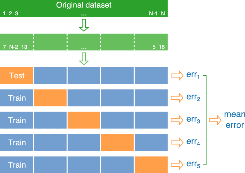
Cross Validation, $L = \ell + k, X^L = X^\ell_n \cup X^k_n$:

$CV(\mu, X^L) = \frac1{|N|} \sum\limits_{n \in N} {Q}(\mu(X^\ell_n), X^k_n) \to \min$

Significant Events in Machine Learning

1997: IBM Deep Blue defeats world chess champion Garry Kasparov

480 chess CPUs
search using alpha-beta pruning modification
two debut books

2004: self-driving cars competition — DARPA Grand Challenge

prize fund of $1 million
in the first race, the winner covered only 11.8 out of 230 km

2006: Google Translate launched

initially statistical machine translation
mobile app appeared in 2010

2011: 40 years of DARPA CALO (Cognitive Assistant that Learns and Organizes) development

Apple's Siri voice assistant launched
IBM Watson won the TV game "Jeopardy!"

2011-2015: ImageNet — error rate reduced from 25% to 3.5% versus 5% in humans

2015: Creation of the open company OpenAI by Elon Musk and Sam Altman, pledged to invest $1 billion

2016: Google DeepMind beat the world champion of the game Go

2018: At the Christie's auction, a painting, formally drawn by AI, sold for $432,500

2020: AlphaFold 2 predicts the structure of proteins with over 90% accuracy for about two-thirds of the proteins in the dataset

2021: DALL-E appears — an AI system developed by OpenAI that can generate images from textual descriptions, which has potential applications in creative industries

2022: ChatGPT (Generative Pre-trained Transformer) developed by OpenAI — fastest-growing consumer software application in history