Machine Learning with Python
Lecture 7. Linear models, Stochastic Gradient Descent
Alexander Avdiushenko
October 24, 2023
Training Regression as Optimization Task
Training sample: $X^\ell = (x_i, y_i)^\ell_{i=1}$, $x_i \in \mathbb{R}^n$, $y_i \in \mathbb{R}$
Linear regression model (weights $w \in \mathbb{R}^n$):
$a(x, w) = \left< w, x\right> = w^T x= \sum\limits_{j=1}^n w_jf_j(x)$
Squared loss function:
$\mathcal{L} (a, y) = (a - y)^2$
Training Method — Least Squares Method:
$Q(w) = \frac1\ell\sum\limits_{i=1}^\ell (a(x_i, w) - y_i)^2 \to \min\limits_w$
Testing on the test set $X^k = (\tilde{x}_i, \tilde{y}_i)_{i=1}^k$:
$\overline{Q}(w) = \frac1k\sum\limits_{i=1}^k (a(\tilde{x}_i, w) - \tilde{y}_i)^2$
Training Classification as Optimization Task
Training sample: $X^\ell = (x_i, y_i)^\ell_{i=1}$, $x_i \in \mathbb{R}^n$, $\ \color{orange}{y_i \in \{-1, +1\}}$
Classification Model — Linear (weights $w \in \mathbb{R}^n$):
$a(x, w) = {\color{orange}\textrm{sign}} \left< w, x\right> = {\color{orange}\textrm{sign}}(\sum\limits_{j=1}^n w_jf_j(x))$Loss Function — Binary or its approximation:
$\mathcal{L} (a, y) = [ay < 0] = [\left< w, x\right> y < 0] \leq \overline{\mathcal{L}}(\left< w, x\right>, y)$Training Method — Minimization of Empirical Risk:
$Q(w) = \frac1\ell\sum\limits_{i=1}^\ell [\left< w, x_i\right> y_i < 0] \leq \frac1\ell\sum\limits_{i=1}^\ell \overline{\mathcal{L}} (\left< w, x_i\right>, y_i) \to \min\limits_w$Testing on the test set: $X^k = (\tilde{x}_i, \tilde{y}_i)_{i=1}^k$
$\overline{Q}(w) = \frac1k\sum\limits_{i=1}^k \color{orange}{[\left<\tilde{x}_i, w\right> \tilde{y}_i < 0]}$The Concept of Margin for Separating Classifiers
Separating classifier:
$a(x, w) = \mathrm{sign}\ g(x, w)$
$g(x, w)$ — separating (discriminant) function, $g(x, w) = 0$ — equation of the separating surface
$M_i(w) = g(x_i, w)y_i$ — margin of object $x_i$
$M_i(w) \leq 0 \iff$ algorithm $a(x, w)$ makes a mistake on $x_i$
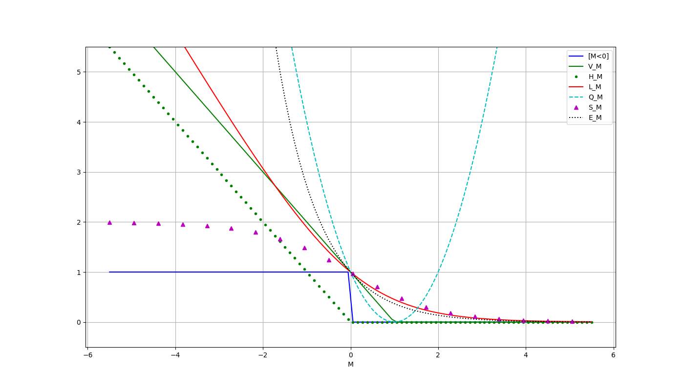
Continuous Approximations of the Threshold Loss Function $\mathcal{L}(M)$
$[M<0]$ — threshold loss function (is not continuous!)
$V(M) = (1 − M)_+$ — piecewise linear (SVM)
$H(M) = (−M)_+$ — piecewise linear (Hebb's rule)
$L(M)=\log_2(1 + \exp(-M))$ — logarithmic (LR)
$Q(M)=(1 − M)^2$ — quadratic
$S(M)=2(1+\exp(M))^{-1}$ — sigmoidal
$E(M)= \exp(-M)$ – exponential (remember for AdaBoost)
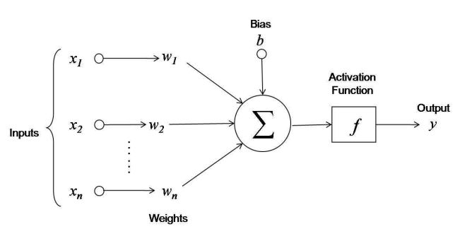
Linear Classifier — Mathematical Model of a Neuron
Linear model of the McCulloch-Pitts neuron, 1943:
$a(x, w) = f(\left< w, x\right>) = f\left(\sum\limits_{j=1}^n w_j x_j - w_0 \right)$
- $f(z)$ — activation function (for example, $\mathrm{sign}$)
- $w_j$ — weight coefficients of synaptic connections
- $w_0 = b$ — activation threshold or bias
- $w, x \in \mathbb{R}^{n+1}$ — if you introduce a constant feature $x_0 \equiv -1$
Gradient Method of Numerical Minimization
Minimization of empirical risk (regression, classification):
$Q(w) = \frac{1}{\ell} \sum\limits_{i=1}^\ell \mathcal{L}_i(w) \to \min\limits_w$Numerical minimization by the gradient descent method:
$w^{(0)} = $ initial approximation
$w^{(t+1)} = w^{(t)} - h \nabla_w Q(w^{(t)})$
where $\nabla_w Q(w) = \left(\frac{\partial Q(w)}{\partial w_j} \right)^n_{j=0}$
$w^{(t+1)} = w^{(t)} - \frac{h}{l} \sum\limits_{i=1}^\ell \nabla_w \mathcal{L}_i(w^{(t)})$
where $h$ is the gradient step, also known as the learning rate
Idea of Speeding up Convergence: take $(x_i, y_i)$ one by one and immediately update the weight vector — stochastic gradient descent.
Visualization of the Gradient Method
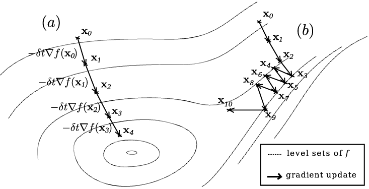
Two possible trajectories of gradient descent:
In version (a), the target function has "good behavior", which allows the point to smoothly move to the optimum by the gradient
In version (b), the gradient begins to oscillate as it falls into a narrow valley, thus converging more slowly
Stochastic Gradient Descent
Input: sample $X^\ell$, learning rate $h$, decay rate $\lambda$
Output: weight vector $w$
- Initialize weights $w_j,\ j = 0, \dots, n$
- Initialize the estimate of the functional: $\overline{Q} = \frac1\ell \sum\limits_{i=1}^\ell \mathcal{L}_i(w)$
- Repeat:
- Select object $x_i$ from $X^\ell$ randomly
- Compute the loss: $\varepsilon_i = \mathcal{L}_i(w)$
- Make a gradient step: $w = w - h \nabla_w \mathcal{L}_i(w)$
- Assess the functional: $\overline{Q} = \lambda \varepsilon_i + (1 - \lambda) \overline{Q}$
Until the value $\overline{Q}$ and/or weights $w$ converge
Robbins, H., Monro S. A stochastic approximation method // Annals of Mathematical Statistics, 1951, 22 (3), p. 400—407.
Recursive Estimate of Error Functional
Problem: Calculating the $Q$ estimate over the entire selection $x_1, \dots, x_\ell$ is much slower than the gradient step for a single object $x_i$
Solution: Use an approximate recursive formula. Arithmetic Mean:
$\overline{Q}_m = \frac1m \varepsilon_m + \frac1m \varepsilon_{m-1} + \frac1m \varepsilon_{m-2} + \dots$
$\overline{Q}_m = {\color{orange}\frac1m} \varepsilon_m + {\color{orange}\left(1 - \frac1m\right)} \overline{Q}_{m-1}$
Exponential Moving Average:
$\overline{Q}_m = \lambda \varepsilon_m + \left(1 - \lambda\right)\lambda\varepsilon_{m-1} + \left(1 - \lambda\right)^2\lambda\varepsilon_{m-2} + \dots$
$\overline{Q}_m = {\color{orange}\lambda} \varepsilon_m + {\color{orange}\left(1 - \lambda\right)} \overline{Q}_{m-1}$
The parameter $\lambda$ is the rate of forgetting the history of the series.
SAG Algorithm (Stochastic Average Gradient)
Input: sample $X^\ell$, learning rate $h$, decay rate $\lambda$
Output: weight vector $w$
- Initialize weights $w_j,\ j = 0, \dots, n$
- Initialize gradients: $G_i = \nabla \mathcal{L}_i(w), i = 1, \dots, \ell$
- Initialize the estimate of the functional: $\overline{Q} = \frac1\ell \sum\limits_{i=1}^\ell \mathcal{L}_i(w)$
- Repeat
- Select object $x_i$ from $X^\ell$ randomly
- Compute the loss: $\varepsilon_i = \mathcal{L}_i(w)$
- Compute the gradient: $G_i = \nabla \mathcal{L}_i(w)$
- Make a gradient step: $w := w - h {\color{orange} \frac1\ell \sum_{i=1}^\ell G_i}$
- Estimate the functional: $\overline{Q} = \lambda \varepsilon_i + (1 - \lambda) \overline{Q}$
Until the value of $\overline{Q}$ and/or weights $w$ converge
Schmidt M., Le Roux N., Bach F. Minimizing finite sums with the stochastic average gradient // arXiv.org, 2013.
Weight Initialization Variants
- $w_j = 0$ for all $j = 0, \dots, n$
- Small random values: $$w_j = \text{random}\left(- \frac{1}{2n}, \frac{1}{2n}\right)$$
- $w_j = \frac{\left< y, f_j \right>}{\left< f_j, f_j \right>}$, where $f_j = (f_j(x_i))_{i=1}^\ell$ — vector of feature values
- The loss function is quadratic, and
- The features are uncorrelated: $\left< f_j, f_k \right> = 0, j \neq k$
- Training on a small random sub-sample of objects
- Multi-start: multiple starts from different random initial approximations and choosing the best solution
This estimate of $w$ is optimal if
Variants of Training Object Order
- Shuffling of objects: alternately take objects from different classes
- More frequently take objects with larger errors: the smaller margin $M_i$, the higher the probability to take the object
- More frequently take objects with lower confidence: the smaller $|M_i|$, the higher the probability to take the object
- Do not take "good" objects at all, for those $M_i > \mu_+$ (this can slightly speed up convergence)
- Do not take outlier objects at all, for those $M_i < \mu_-$ (this can potentially improve classification quality)
You will have to adjust the parameters $\mu_+, \mu_-$
Variants of Gradient Step Selection
- Convergence is guaranteed (for convex functions) when
- The method of fastest gradient descent:
- Test random steps for "knocking out" the iterative process from local minima
- The Levenberg-Marquardt method (second order)
$$h_t \to 0, \sum\limits_{t=1}^{\infty} h_t = \infty, \sum\limits_{t=1}^{\infty} h_t^2 < \infty,$$
in particular, you can set $h_t = 1/t$
$$\mathcal{L}_i(w - h\nabla \mathcal{L}_i(w)) \to \min\limits_h$$
allows you to find an adaptive step $h^*$. For a quadratic loss function, $h^* = \|x_i\|^{-2}$
Levenberg-Marquardt Diagonal Method
Newton-Raphson method, $\mathcal{L}_i(w) \equiv \mathcal{L}(\left< w, x_i\right>y_i)$:
$w = w - h(\mathcal{L}_i^{\prime\prime}(w))^{-1} \nabla \mathcal{L}_i(w)$
where $\mathcal{L}_i^{\prime\prime}(w) = \left( \frac{\partial^2\mathcal{L}_i(w)}{\partial w_j \partial w_k} \right)$ — hessian, an $n\times n$ matrix
Heuristic. We assume that the hessian is diagonal:
$w_j = w_j - h\left(\frac{\partial^2\mathcal{L}_i(w)}{\partial w_j^2} + \mu\right)^{-1} \frac{\partial \mathcal{L}_i(w)}{\partial w_j}$,
$h$ — learning rate, we can assume $h = 1$
$\mu$ — parameter that prevents zeroing of the determinant
The ratio $h/\mu$ is the learning rate on flat parts of the functional $\mathcal{L}_i(w)$, where the second derivative is zeroed out.
Overfitting Problem
Possible reasons for overfitting:
- Too few objects and too many features
- Linear dependence (multicollinearity) of features:
- Suppose a classifier has been built: $a(x, w) = \mathrm{sign} \left< w, x\right>$
- Multicollinearity: $\exist u \in \mathbb{R}^{n+1}: \forall x_i \in X^\ell \left< u, x_i\right> = 0$
- Non-uniqueness of the solution: $\forall \gamma \in \mathbb{R}\ a(x, w) = \mathrm{sign} \left< w + \gamma u, x\right>$
Manifestations of overfitting:
- Too large weights $|w_j|$ of different signs
- Instability of the discriminant function $\left< w, x\right>$
- $Q(X^\ell) \lt\lt Q(X^k)$
Main way to reduce overfitting:
Regularization (weight decay)
Regularization (weight decay)
Penalty for increasing the norm of the weight vector:
$\mathcal{\tilde L}_i(w) = \mathcal{L}_i(w) + \frac{\tau}{2} \|w\|^2 = \mathcal{L}_i(w) + \frac{\tau}{2}\sum\limits_{j=1}^n w_j^2 \to \min\limits_w$
Gradient: $\nabla \mathcal{\tilde L}_i(w) = \mathcal{\tilde L}_i(w) + \tau w$
Modification of the gradient step:
$w = w{\color{orange}(1 - h\tau)} - h \nabla \mathcal{L}_i(w)$
Methods for selecting the regularization coefficient $\tau$:
- sliding control
- stochastic adaptation
- two-level Bayesian inference
SG: advantages and disadvantages
Advantages:
- easy to implement
- easy to generalize to any $g(x, w), \mathcal{L}(a, y)$
- easy to add regularization
- possible dynamic (streaming) learning
- on super-large samples, you can get a decent solution, even without processing all $x_i, y_i$
- suitable for tasks with large data
Disadvantages:
- selection of a complex of heuristics is an art (do not forget about overfitting, getting stuck, divergence)
Principle of maximum likelihood
Let $X \times Y$ be a probability space, and the model (i.e., its parameters $w$) is also generated by some probability distribution.
Bayes' theorem:
$P(A|B) = \frac{P(B|A)P(A)}{P(B)}$
$A \equiv w$, $B \equiv Y, X\ \Rightarrow$
$P(w|Y, X) = \frac{P(Y, X|w)P(w)}{P(Y, X)} = \frac{P(Y | X, w)P(X|w)P(w)}{P(Y | X)P(X)}$
$\boxed{P(w|Y,\ X) = \frac{P(Y|w, X)P(w)}{P(Y | X)}}$
Here:
$P(w|Y, X)$ — posterior distribution of parameters
$P(Y|X, w)$ — likelihood
$P(w)$ — prior distribution of parameters
Connection of likelihood and approximation of empirical risk
Maximum likelihood
$L(w) = \sum\limits_{i=1}^\ell {\color{orange}\log P(y_i|w, x_i)} \to \max\limits_w$
Minimization of the approximated empirical risk
$Q(w) = \sum\limits_{i=1}^\ell {\color{orange}\mathcal{L}(y_i, x_i, w)} \to \min\limits_w$
These two principles are equivalent if we set
$ -\log P(y_i|w, x_i) = \mathcal{L}(y_i, x_i, w)$
Model $P(y|x,w) \equiv $ Model $g(x,w)$ and $\mathcal{L}(M)$
Probabilistic interpretation of regularization
\(P(y|x, w)\) — probabilistic data model
\(P(w; \gamma)\) — prior distribution of model parameters, \(\gamma\) — vector of hyperparameters;
Joint likelihood of data and model
\[P(X^\ell, w) = P(X^\ell | w)P(w;\gamma)\]Maximum a Posteriori Probability (MAP) principle:
\[ L(w) = \log P(X^\ell, w) = \sum\limits_{i=1}^\ell \log P(y_i|w, x_i) + \underbrace{\color{orange}{\log P(w; \gamma)}}_{\text{regularizer}} \to \max\limits_w \]How else can the logarithm help?
Examples: Gaussian and Laplace priors
Let the weights \(w_j\) be independent, \(Ew_j = 0\), \(Dw_j = С\)
Gaussian distribution and quadratic (\(L_2\)) regularizer:
$$P(w; С) = \frac{1}{(2\pi C)^{n/2}} \exp \left(-\frac{{\|w\|^2_2}}{2C}\right)$$ $${\|w\|^2_2 = \sum\limits_{j=1}^n w_j^2}$$ $$-\log P(w; С) = \frac{1}{2C}\|w\|^2_2 + const$$Laplace distribution and absolute (\(L_1\)) regularizer:
$$P(w; С) = \frac{1}{(2C)^{n}} \exp \left(-\frac{{\|w\|_1}}{C}\right)$$ $${\|w\|_1 = \sum\limits_{j=1}^n |w_j|}$$ $$-\log P(w; С) = \frac{1}{C}\|w\|_1 + const$$\(C\) — hyperparameter, \(\tau = \frac{1}{C}\) — regularization coefficient
Binary Logistic Regression
-
Linear classification model for two classes \(Y = \{-1, 1\}\):
\(a(x) = \mathrm{sign} \left< w, x\right>\), \(x, w ∈ \mathbb{R}^n\), margin \(M = \left< w, x\right>y\) - Logarithmic loss function: $$\mathcal{L}(M) = \log(1 + e^{-M})$$
- Conditional probability model: $$ P(y|x, w) = \sigma(M) = \frac{1}{1 + e^{-M}},$$ where \(\sigma(M)\) is the sigmoid function, important property: \(\sigma(M) + \sigma(-M) = 1\)
- Regularized logistic regression learning problem (minimization of approximated empirical risk): $$Q(w) = \sum\limits_{i=1}^\ell \log(1 + \exp(-\left< w, x_i\right>y_i)) + \frac{\tau}{2}\|w\|^2_2 \to \min\limits_w $$
Multiclass Logistic Regression
Linear classifier with an arbitrary number of classes \(|Ү|\):
\(a(x) = \arg\max\limits_{y \in Y} < w_y, x>\), \(x, w_y \in \mathbb{R}^n\)The probability that the object \(x\) belongs to the class \(y\):
\(P(y|x,w) = \frac{\exp< w_y, x>}{\sum\limits_{z \in Y} \exp< w_z, x>} = \underset{y \in Y}{\mathrm{softmax}} < w_y, x>\)The \(\mathrm{softmax}: \mathbb{R}^Y \to \mathbb{R}^Y\) function converts any vector into a normalized vector of a discrete distribution.
Maximization of likelihood (log-loss) with regularization:
\( L(w) = \sum\limits_{i=1}^\ell \log P(y_i|w, x_i) - \frac{\tau}{2} \sum\limits_{y \in Y} \|w_y\|^2 \to \max\limits_w \)Summary
- The Stochastic Gradient (SG, SAG) method is suitable for any models and loss functions
- Well suited for large data learning
- Approximation of the threshold loss function $\mathcal{L}(M)$ allows the use of gradient optimization
- Functions $\mathcal{L}(M)$, penalizing for the approximation to the class boundary, increase the gap between classes, thereby improving classification reliability
- Regularization solves the multicollinearity problem and also reduces overfitting
- Likelihood maximization and minimization of the empirical risk are different views on the same optimization problem