Machine Learning with Python
Lecture 11. Ensembles, random forest and gradient boosting
Alex Avdiushenko
November 7, 2023
Notations
$X^\ell = (x_i, y_i)^\ell_{i=1} \subset X \times Y$ — training set, $y_i = y^*(x_i)$
$a(x) = C(b(x))$ — algorithm, where
$b: X \to {R}$ — base algorithm (operator)
$C: {R} \to Y$ — decision rule (composition)
${R}$ — space of estimates
Definition
Ensemble of base algorithms \(b_1, \dots, b_T\)
\(a(x) = C(F(b_1(x), \dots, b_T(x)))\)
where \(F: R^T \to R\) — correcting operation
Why introduce correcting operation \(R\)?
In classification tasks, the set of mappings \(\{F: R^T \to R\}\) is significantly wider than \(\{F: Y^T \to Y\}\)
Examples of Evaluation Spaces and Decision Rules
- Example 1: binary classification, \(Y = \{-1, +1\}\): \[a(x) = \text{sign}(b(x))\] so \(R = \mathbb{R}, b: X \to \mathbb{R}, C(b) = \text{sign}(b)\)
- Example 2: multiclass classification with \(M\) classes \(Y = \{1,\dots, M\}\): \[a(x) = \arg\max_{y \in Y} b_y(x)\] so \(R = \mathbb{R}^M, b: X \to \mathbb{R}^M, C(b_1, \dots, b_M) \equiv \arg \max_{y \in Y} b_y\)
-
Example 3: regression, \(Y = R = \mathbb{R}\)
\(C(b) \equiv b\) — there is no need for a decision rule
Examples of Ensembles (Correcting Operations)
-
Example 1: Simple Voting
\(F(b_1(x),\dots, b_T(x)) = \frac{1}{T} \sum\limits_{t=1}^T b_t(x), x \in X\) -
Example 2: Weighted Voting
\(F(b_1(x),\dots, b_T(x)) = \sum\limits_{t=1}^T \alpha_tb_t(x), x \in X, \alpha_t \in \mathbb{R}\) -
Example 3: Mixture of Experts
\(F(b_1(x),\dots, b_T(x)) = \sum\limits_{t=1}^T g_t(x)b_t(x), x \in X, g_t: X \to \mathbb{R}\)
Stochastic Methods for Building Compositions
To make sure the algorithms in the composition are distinct:
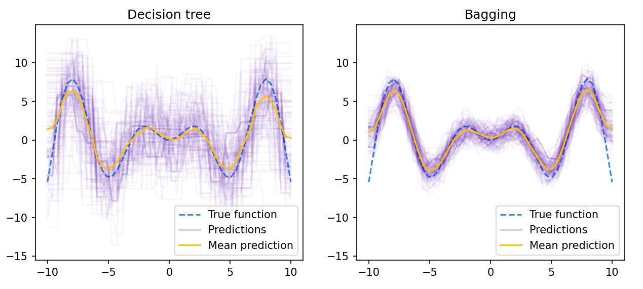
- They are trained on (random) sub-samples
— bagging = bootstrap aggregation. [Breiman, 1996]: sub-samples of length \(\ell\) with repetitions. Ratio of objects falling into the sample \(\left( 1 - \frac{1}{e}\right) \approx 0.632\) - Or on (random) subsets of features
— RSM = random subspace method, [Ho, 1998]
Boosting explained
Boosting for binary classification tasks
Let's take \(Y = \{\pm 1\}, b_t: X \to \{-1, {\color{orange}[0]}, +1\}, C(b) = \text{sign}(b)\)
Weighted voting
\(a(x) = \text{sign}\left( \sum\limits_{t=1}^T \alpha_t b_t (x)\right), x \in X\)
Quality functional of composition
Number of errors in \(X^\ell\): \(Q_T = \sum\limits_{i=1}^\ell \left[y_i \sum\limits_{t=1}^T \alpha_t b_t(x_i) < 0 \right]\)
Two main boosting heuristics:
- Fix \(\alpha_1 b_1(x), \dots, \alpha_{t-1} b_{t-1}(x)\) when adding \(\alpha_{t}b_t(x)\)
- Smooth approximation of the threshold loss function \([M < 0]\)
Exponential Approximation of the Threshold Loss Function
The quality functional \(Q_T\) is estimated from above:
\[Q_T \leq \tilde Q_T = \sum_{i=1}^\ell \underbrace{\exp(-y_i \sum_{t=1}^{T-1} \alpha_t b_t (x_i))}_{w_i} \exp(-y_i \alpha_T b_T (x_i))\]Normalized weights: \[\tilde W^\ell = (\tilde w_1, \dots, \tilde w_\ell), \tilde w_i = w_i / \sum\limits_{j=1}^\ell w_j\]
Weighted number of erroneous (negative) and correct (positive) classifications for weights vector \(U^\ell = (u_1, \dots, u_\ell)\):
\(N(b, U^\ell) = \sum\limits_{i=1}^\ell u_i [b(x_i) = -y_i]\)
\(P(b, U^\ell) = \sum\limits_{i=1}^\ell u_i [b(x_i) = y_i]\)
\((1 - N - P)\) — weighted number of classification refusals
Classical Variant of AdaBoost
Assume there are no rejections, \(b_t: X \to \{\pm 1 \}\). Then \(P = 1 − N\)
Theorem (Freund, Schapire, 1995)
Suppose that for any normalized weight vector \(U^\ell\) there exists an algorithm \(b \in B\), classifying the sample at least slightly better than at random: \(N(b, U^\ell) < \frac12\).
Then the minimum of the functional \(\tilde Q_T\) is reached when
\[b_T = \arg\min_{b \in B} N (b, \tilde W^\ell), \quad \alpha_T = \frac12 \ln\frac{1-N(b_T, \tilde W^\ell)}{N(b_T, \tilde W^\ell)}\]AdaBoost Algorithm
Input: Training sample \(X^\ell\), parameter \(T\)
Output: Base algorithms and their weights \(\alpha_t b_t, t = 1, \dots, T\)
- Initialize object weights: \(w_i = \frac{1}{\ell}, i = 1, \dots, \ell\)
- for all \(t = 1, \dots, T\)
- Update object weights: \(w_i = w_i \exp(-\alpha_t y_i b_t(x_i)), i = 1, \dots, \ell\)
- Normalize object weights: \[ w_0 = \sum_{j=1}^\ell w_j ,\ w_i = w_i / w_0, i = 1, \dots, \ell\]
Train the basic algorithm: \(b_t = \arg \min\limits_b N(b, W^\ell)\)
\(\alpha_t = \frac12 \ln \frac{1-N(b, W^\ell)}{N(b, W^\ell)}\)
Heuristics and Recommendations
-
Base classifiers (weak classifiers)
- Decision trees — most commonly used
- Threshold rules (data stumps)
\(B = \{b(x) = [f_j(x) \lessgtr\theta] | j = 1, \dots, n, \theta \in \mathbb{R}\}\) - For strong classifiers (as SVM for instance), boosting is usually not effective
- Noise rejection: dispose of objects with the largest \(w_i\)
- Additional stop criterion: increase in error rate on the validation set
Drawbacks of AdaBoost
- Over-sensitivity to outliers due to $e^M$
- AdaBoost creates "black boxes" — cumbersome, not interpretable compositions of hundreds of algorithms
- It requires fairly large training sets (Bagging can manage with shorter ones)
Ways to eliminate:
- Other approximations to the threshold loss function
- Continuous real base algorithms $b_t: X \to \mathbb{R}$
- Explicit optimization of margins, without approximation
- Less greedy strategies for growing the composition
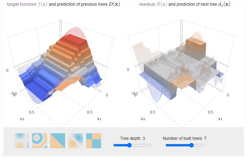
Gradient Boosting for Arbitrary Loss Function (GB machine)
Linear (convex) combination of base algorithms:
\[a(x) = \sum\limits_{t=1}^T \alpha_t b_t(x), \ x \in X, \ \alpha_t \in \mathbb{R}_+\]Quality functional with arbitrary loss function $\mathcal{L}(a, y)$:
\[Q(\alpha, b, X^\ell) = \sum\limits_{i=1}^\ell \mathcal{L} \underbrace{\overbrace{(\sum\limits_{t=1}^{T-1} \alpha_t b_t(x_i)}^{f_{T-1,i}} + \alpha b(x_i)}_{f_{T,i}} , y_i) \to \min\limits_{\alpha, b}\]$f_{T-1, i}$ — current approximation, $f_{T, i}$ — next approximation
Parametric approximation of the gradient step
Gradient method of minimization $Q(f) \to \min, f \in \mathbb{R}^\ell$:
$f_0 =$ initial approximation
$f_{T,i} = f_{T-1,i} - \alpha g_i, \ i = 1, \dots, \ell$
$g_i = \mathcal{L}^\prime (f_{T-1, i}, y_i)$ — components of the gradient vector, $\alpha$ — gradient step
Observation: this is very similar to one boosting iteration!
$f_{T,i} = f_{T-1,i} + \alpha b(x_i), \ i = 1, \dots, \ell$
Idea: we will look for such a basic algorithm $b_T$ that the vector $(b_T(x_i))_{i=1}^\ell$ will approximate the antigradient vector $(-g_i)_{i=1}^\ell$ $$b_T = \arg\min\limits_b \sum\limits_{i=1}^\ell (b(x_i) + g_i)^2$$Gradient Boosting Algorithm
Input: training set $X^\ell$, parameter $T$
Output: base algorithms and their weights $\alpha_t b_t, t = 1, \dots, T$
- Initialization: $f_i = 0, i = 1, \dots, \ell$
- for all $t = 1, \dots, \color{orange}{T}$
- One-dimensional minimization problem: $\alpha_t = \arg \min\limits_{\alpha > 0} \sum\limits_{i=1}^\ell \mathcal{L}(f_i + \alpha b_t(x_i), y_i)$
- Updating the vector of values on the sample objects: $f_i = f_i + \alpha_t b_t(x_i)), i = 1, \dots, \ell$
Basic algorithm approximating antigradient:
$$b_t = \arg \min\limits_b \sum\limits_{i=1}^\ell (b(x_i) + \mathcal{L}^\prime(f_i, y_i))^2$$Stochastic Gradient Boosting (SGB)
Idea: In steps 2-4, use not the entire sample \(X^\ell\), but a random subsample without replacement.
Advantages:
- Improved quality
- Enhanced convergence
- Reduced training time
Friedman G. Stochastic Gradient Boosting, 1999
Regression and AdaBoost
Regression: \(\mathcal{L}(a,y) = (a-y)^2\)
- \(b_T(x)\) is trained on differences \(y_i - \sum\limits_{t=1}^{T-1} \alpha_t b_t (x_i)\)
- If regression is linear, then \(\alpha_t\) doesn't need to be trained
Classification: \(\mathcal{L}(a,y) = e^{-ay}, b_t \in \{-1, 0 , +1\}\)
- GB exactly matches AdaBoost
XGBoost — a popular and fast implementation of gradient boosting over trees
Regression and classification trees (CART):
$$b(x) = \sum\limits_{j=1}^J w_j [x \in R_j]$$where $R_j$ is the area of space covered by leaf $j$, $w_j$ is the leaf weights, and $J$ is the number of leaves in the tree.
Quality functional with a total of $L_0, L_1, L_2$ regularizers:
$Q(b, \{w_j\}_{j=1}^J, X^\ell) = \sum\limits_{i=1}^\ell \mathcal{L} \left(\sum\limits_{t=1}^{T-1} \alpha_t b_t(x_i) + \alpha b(x_i, y_i)\right) + \gamma \sum\limits_{j=1}^J [w_j \neq 0] + \mu \sum\limits_{j=1}^J |w_j| + \frac{\lambda}{2} \sum\limits_{j=1}^J w_j^2 \to \min\limits_{b, w_j}$The task has an analytic solution for $w_j$.
Other popular implementations of gradient boosting over random trees: LightGBM, CatBoost
Summary of ensembles
- Ensembles allow solving complex tasks that are poorly solved by individual algorithms
- It's too difficult to train the ensemble as a whole. Therefore, we train basic algorithms one by one
- An important discovery in the mid-90s: boosting's generalizing ability doesn't worsen with the increasing complexity $T$
- Gradient boosting — the most general of all boostings:
- an arbitrary loss function
- an arbitrary space of estimates $R$
- suitable for regression, classification, ranking
- Its stochastic version SGB — better and faster
- Most often, GB is applied to decision trees
- Gradient boosting over Oblivious Decision Trees with categorical features = Catboost
Comparison: boosting — bagging — RSM
- Boosting is better for large training datasets and classes with complex shape borders
- Bagging and RSM are better for small training datasets
- RSM is better in cases where there are more features than objects, or when there are many non-informative features
- Bagging and RSM can be effectively parallelized, boosting is performed strictly sequentially

Random Forest
Training a random forest:
- Bagging over decision trees, without pruning
- The feature in each tree node is chosen from a random subset of $k$ out of $n$ features
The number of trees $T$ can be selected based on the out-of-bag criterion — the number of errors on objects $x_i$, if we don't consider the votes of trees for which $x_i$ was training:
$$\text{out-of-bag}(a) = \sum\limits_{i=1}^\ell \left[\text{sign}(\sum\limits_{t=1}^T [x_i \notin U_t] b_t(x_i)) \neq y_i \right] \to \min$$This is an unbiased estimate of generalization ability.
Justification of Boosting
Strengthening the concept of the error rate of the algorithm $a(x) = \text{sign}(b(x))$
$$\nu_\theta (a, X^\ell) = \frac{1}{\ell} \sum\limits_{i=1}^\ell [b(x_i) y_i \leq \theta]$$The usual error rate $\nu_0 (a, X^\ell) \leq \nu_\theta (a, X^\ell)$ when $\theta > 0$
Theorem (Freund, Schapire, Bartlett, 1998)
If $|B| < \infty$, then $\forall \theta > 0, \forall \eta \in (0,1)$ with a probability $1-\eta$
$$P[y a(x) < 0] \leq \nu_\theta (a, X^\ell) + C\sqrt{\frac{\ln |B| \ln \ell}{\ell\theta^2} + \frac{1}{\ell}\ln \frac{1}{\eta}}$$Main conclusion
The estimate depends on $|B|$, but not on $T$. Voting does not increase the complexity of the effectively used set of algorithms.
Justification of Boosting: what is actually happening?
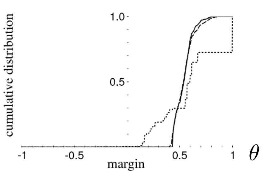
Distribution of margins: the share of objects with a margin smaller than a fixed $\theta$ after 5, 100, 1000 iterations (UCI classification task: vehicle)
- With growing $T$, the margin distribution shifts to the right, that is, boosting "spreads" the classes in the space of growing-dimension vectors $(b_1(x), \dots, b_T(x))$
- Therefore, the second term can be reduced in the estimate by increasing $\theta$ and not changing $\nu_\theta (a, X^l)$
- The second term can be reduced if |B| is reduced, that is, if a simple family of basic algorithms is taken