Machine Learning with Python
Lecture 9. Logical Rules and Decision Trees
Alex Avdiushenko
October 31, 2023
Logical rule
$X^\ell = (x_i, y_i)_{i=1}^\ell \subset X \times Y$ — training sample, $y_i = y(x_i)$
A logical rule (regularity) is a predicate $R: X \in \{0, 1\}$, satisfying two requirements:
- Interpretability:
- $R$ is written in natural language
- $R$ depends on a small number of features (usually 1-7)
- Informativeness with respect to one of the classes $c \in Y$:
- $p_c (R) = #\{x_i : R(x_i)=1 \text{ and } y_i =c\} \to \max$
- $n_c (R) = #\{x_i : R(x_i)=1 \text{ and } y_i \neq c\} \to \min$
If $R(x) = 1$, then we say "$R$ covers $x$"
Example (from the medical field)
If "age > 60" and "patient has previously had a heart attack", then do not perform surgery, the risk of negative outcome is 60%
Example (from the field of corangeit scoring)
If "home phone is listed on the form" and "salary > $2000" and "loan amount < $5000" then the loan can be issued, default risk is 5%
Main steps of rules induction
- Selection of rule family for finding regularities
- Rule generation
- Rule regularity selection
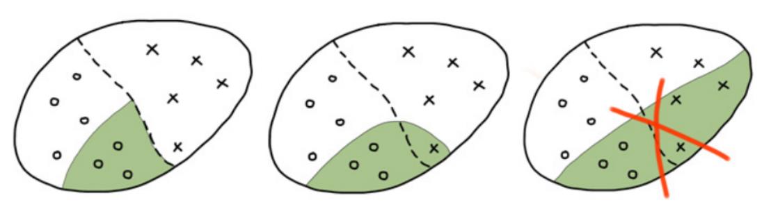
A regularity is a highly informative, interpretable, single-class classifier with rejections.
Rule family selection
- Threshold condition (decision stump): $$R(x) = [f_j(x) \leq {\color{orange}a_j}] \text{ or } [{\color{orange}a_j} \leq f_j(x) \leq {\color{orange}b_j}]$$
- Conjunction of threshold conditions: $$R(x) = \bigwedge\limits_{j \in {\color{orange}J}} [{\color{orange}a_j} \leq f_j(x) \leq {\color{orange}b_j}]$$
- Syndrome — at least $d$ conditions out of $|J|$ must hold (for $d = |J|$ this is conjunction, for $d = 1$ — disjunction):
Parameters ${\color{orange}J, a_j, b_j, d,}$ are tuned using the training set via optimization of the information criterion.
- Half-plane — linear threshold function: $$R(x) = \left[\sum\limits_{j \in {\color{orange}J}} {\color{orange}w_j} f_j(x) \geq {\color{orange}w_0}\right]$$
- Sphere — proximity threshold function: $$R(x) = [(\rho(x, {\color{orange}x_0}) \leq {\color{orange}w_0}]$$
- AVE — algorithms for calculating estimates [Yu. I. Zhuravlev, 1971]: $$\rho(x, {\color{orange}x_0}) = \max\limits_{j \in {\color{orange}J}} {\color{orange}w_j} |f_j(x) - f_j({\color{orange}x_0})|$$
- SCM — set covering machine [M. Marchand, 2001]:
Parameters ${\color{orange}J, w_j, w_0, x_0, \gamma,}$ are tuned using the training set via optimization of the information criterion.
Rules generation
Input: Training sample $X^\ell$
Output: Set of rules $Z$
- Initial set of rules $Z$
- repeat
- $Z^\prime :=$ set of local modifications of the rules $R \in Z$
- remove overly similar rules from $Z \cup Z^\prime$
- $Z :=$ most informative rules from $Z \cup Z^\prime$
- until the rules keep improving
- return $Z$
Specific cases of optimization
- Genetic (evolutionary) algorithms
- Guided Local Search (GLS) — adjusting penalties during the search process
- Branch and bound method — discarding areas that definitely do not contain optimal solutions
Local rule modifications
Example. Family of conjunctions of threshold conditions:
$$ R(x) = \bigwedge\limits_{j \in {\color{orange}J}} [{\color{orange}a_j} \leq f_j(x) \leq {\color{orange}b_j}]$$Local modifications of a conjunctive rule:
- varying one of the thresholds ${\color{orange}a_j}$ or ${\color{orange}b_j}$
- varying both thresholds ${\color{orange}a_j}$ and ${\color{orange}b_j}$ simultaneously
- adding feature ${\color{orange}f_j}$ to ${\color{orange}J}$ with variation of thresholds ${\color{orange} a_j, b_j}$
- removing feature ${\color{orange}f_j}$ from ${\color{orange}J}$
- When removing a feature (pruning), informativeness is usually evaluated on a control sample (hold-out)
- The same methods are suitable for optimizing the set $J$ as for feature selection
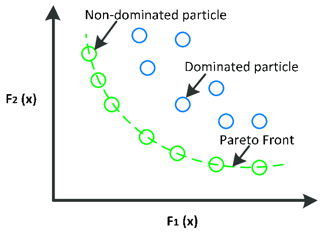
Regularity selection based on pair of criteria $p_c \to \max, n_c \to \min$
Pareto front — a set of non-improvable regularities. A point is non-improvable if there are no points to the left and below it.
Problem: it would be desirable to have a single scalar criterion.
Complex informativeness criteria
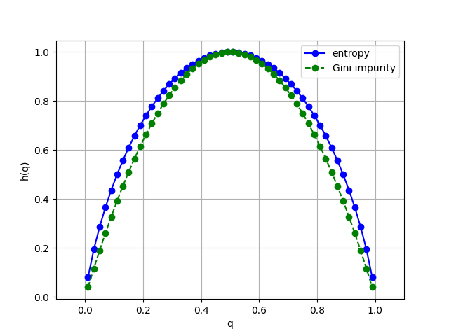
- Entropy information gain criterion:
$ IGain(p, n) = h\left(\frac{P}{\ell} \right) - \frac{p+n}{\ell} h\left(\frac{p}{p+n} \right) - \frac{\ell-p-n}{\ell} h\left(\frac{P-p}{\ell-p-n} \right) \to \max $
$ h(q) = -q \log_2 q - (1-q) \log_2 (1 - q)$ — entropy of “two-class distribution”
- Gini Impurity:
$IGini(p, n) = IGain(p, n)$ when $h(q) = 4q(1 - q)$
- Fisher's Exact Test:
$IStat(p, n) = -\frac{1}{\ell} \log_2 \frac{C_P^pC_N^n}{C_{P+N}^{p+n}} \to \max$ — this is simply the probability of realizing such a pair of $p, n$
- Boosting criterion [Cohen, Singer, 1999]: $$\sqrt{p} - \sqrt{n} \to \max$$
- Normalized boosting criterion: $$\sqrt{\frac{p}{P}} - \sqrt{\frac{n}{N}} \to \max$$
Combined use of regularities
- Weighted Voting (linear classifier with weights $w_{yt}$): $$a(x) = \arg\max_{y \in Y} \sum_{t=1}^{T} w_{yt} R_{yt}(x)$$
- Simple Voting (majority committee): $$a(x) = \arg\max_{y \in Y} \frac{1}{T_y}\sum_{t=1}^{T_y} R_{yt}(x)$$
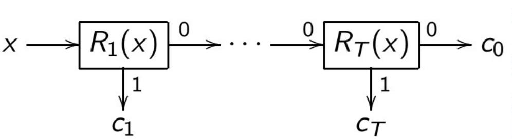
- Decision List (seniority committee), \(c_t \in Y \):
Decision Tree
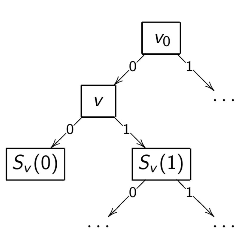
A decision tree is a classification algorithm $a(x)$, defined by a tree (a connected acyclic graph).
- $V = V_{\text{internal}} \cup V_{\text{leaf}}, v_0 \in V$ — root of the tree
- $v \in V_{\text{internal}}:$ functions $f_v: X \to D_v$ and $S_v: D_v \to V, |D_v| < \infty$
- $v \in V_{\text{leaf}}:$ label of the class $y_v \in Y$
Special case: $D_v = {0, 1}$ — binary decision tree
Example: $f_v(x) = [f_j(x) \ge \theta_j]$
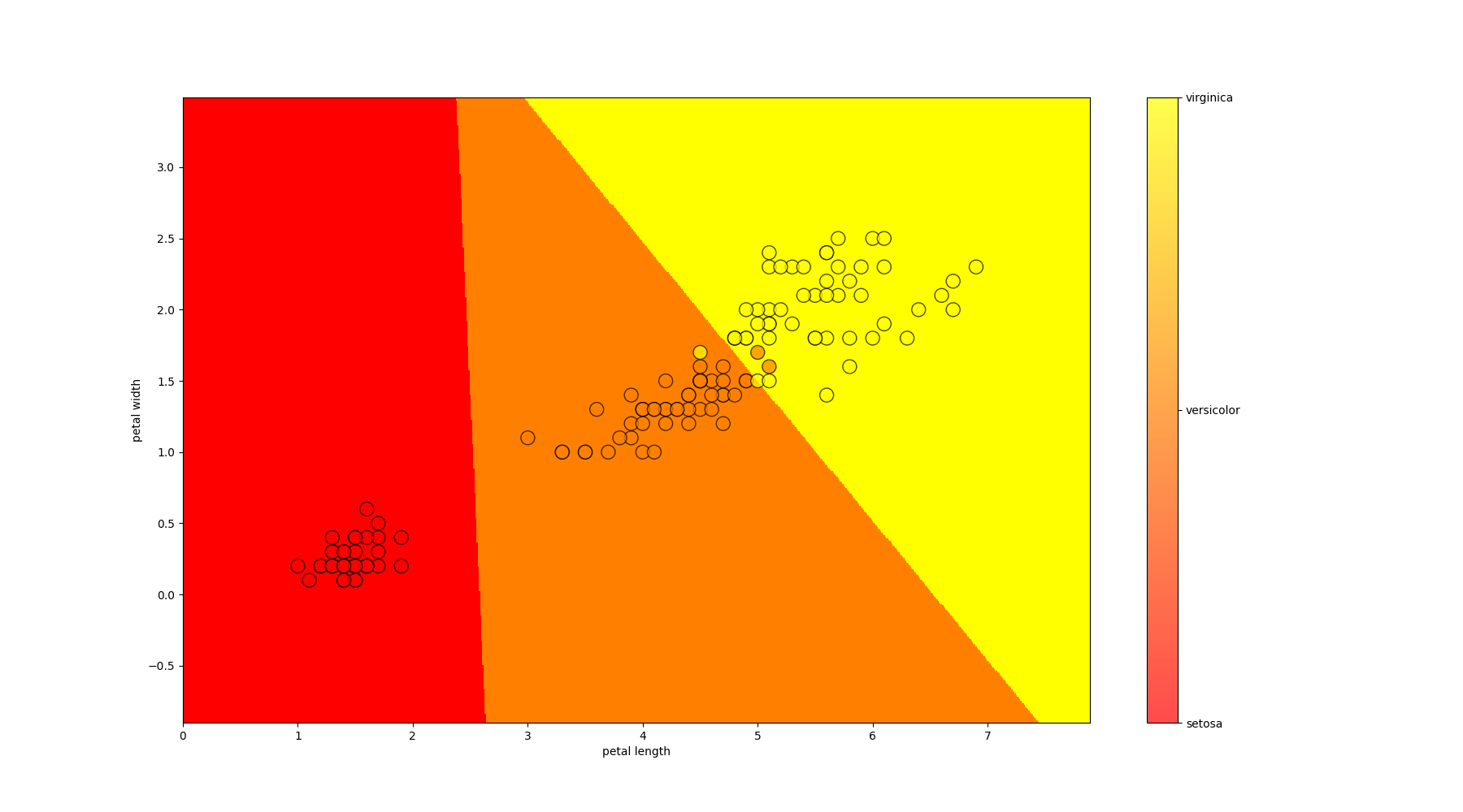
Fisher's Iris
A simple well-known dataset for classification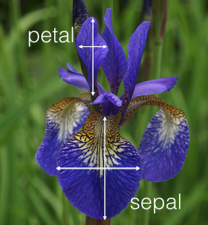
Classes:
- Iris setosa
- Iris virginica
- Iris versicolor
Features:
- Length/Width of the sepal
- Length/Width of the petal
Let's write a function to train on data, predict the answer for each lattice point, and visualize the result. Because the data is much better divided by petals; we visualize only them (we take the average parameters of the sepals)
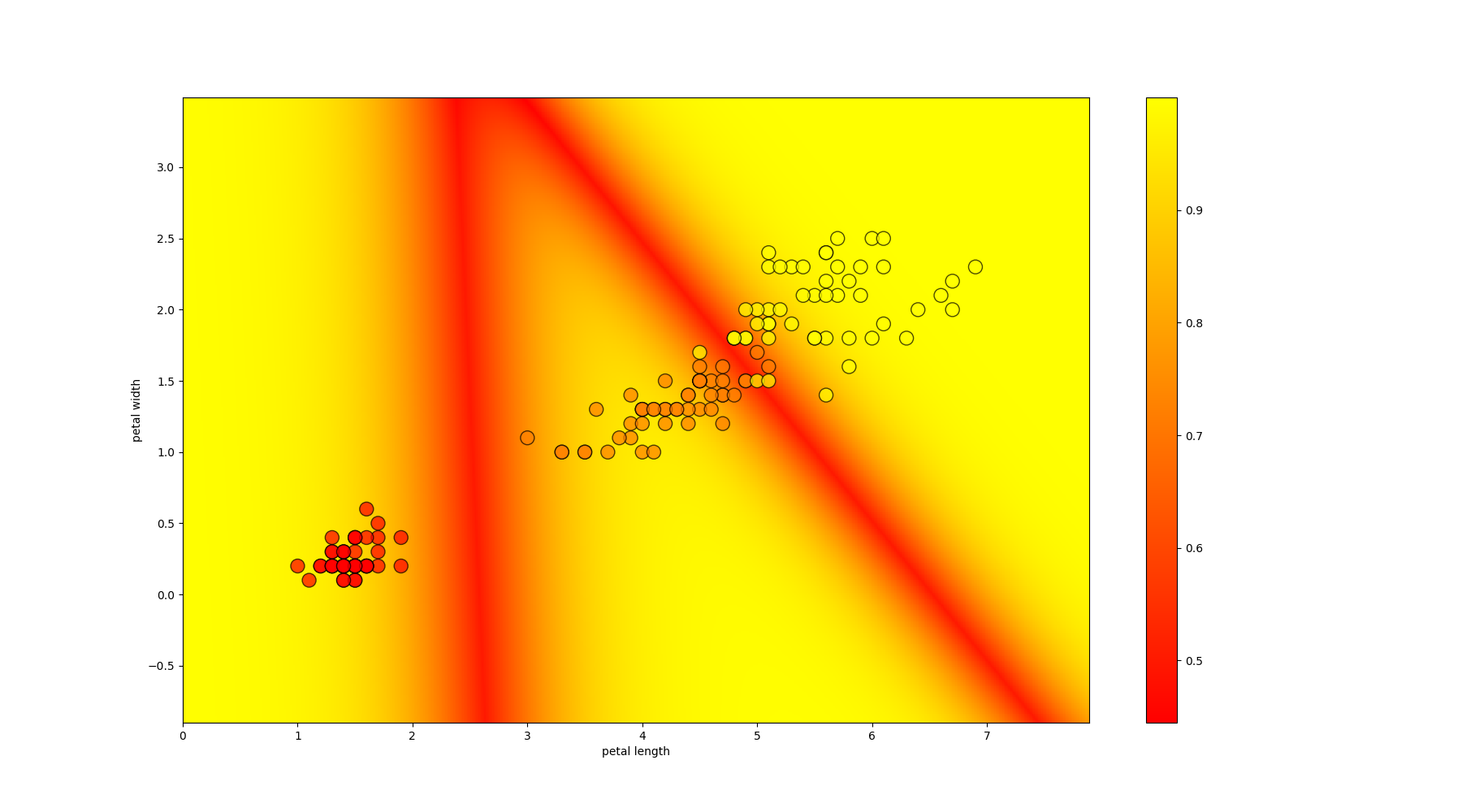
Decision Tree Classifier
Training a Decision Tree: ID3 Algorithm
$v_0$ := TreeGrowing($X_\ell$)
- FUNCTION TreeGrowing($U \subseteq X_\ell$) $\mapsto$ root of a tree $v$
- if StopCriteria($U$) then
return a new leaf $v$, taking $y_v$ := Major*($U$) - find the most profitable feature for branching the tree: $f_v$ = $\arg\max\limits_{f \in F}$ Gain($f, U$)
- if Gain ($f_v$, $U$) < $G_0$ then
return a new leaf $v$, taking $y_v$ := Major($U$) - create a new internal node $v$ with the function $f_v$
- for all $k \in D_v$ $U_k = \{x \in U: f_v(x) = k\}, S_v(k)$ := TreeGrowing($U_k$)
- return $v$
Majority rule: Major($U$) := $\arg\max P(y|U)$
Measure of Uncertainty of Distribution
The frequency estimate of the class \(y\) at the node \(v \in V_{\text{internal}}\):
\[ p_y \equiv P(y|U) = \frac{1}{|U|} \sum\limits_{x_i \in U} [y_i = y] \]
\(\Phi(U)\) — measure of uncertainty (impurity) of the distribution \(p_y\):
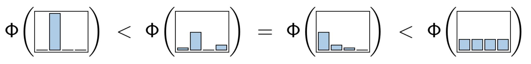
- is minimal, when \(p_y \in \{0,1\}\)
- is maximal, when \(p_y = \frac{1}{|Y|}\) for all \(y \in Y\)
- is symmetrical: does not depend on the renumbering of classes
where \(\mathcal{L}(p)\) decreases and \(\mathcal{L}(1) = 0\), for example: \(-\log p, 1-p, 1-p^2\)
Branching Criterion
The uncertainty of the distributions \(P(y_i | U_k)\) after branching the node \(v\) using the feature \(f\) and partitioning \[U = \bigsqcup\limits_{k \in D_v} U_k\]
\[ \Phi(U_1, \dots , U_{|D_v|}) = \frac{1}{|U|} \sum\limits_{x_i \in U} \mathcal{L}(P(y_i| U_{f(x_i)})) = \\ = \frac{1}{|U|} \sum\limits_{k \in D_v} \sum\limits_{x_i \in U_k} \mathcal{L}(P(y_i| U_{k})) = \sum\limits_{k \in D_v} \frac{|U_k|}{|U|} \Phi(U_k) \]
The gain from branching the node \(v\):
\[ \text{Gain} (f, U) = \Phi(U) - \Phi(U_1, \dots , U_{|D_v|}) = \Phi(U) - \sum\limits_{k \in D_v} \frac{|U_k|}{|U|} \Phi(U_k) \to \max\limits_{f \in F} \]Gini and Entropy Criteria
Two classes, \(Y = \{0, 1\}\), \(P(y|U) = \begin{cases} q, &y = 1 \\ 1-q, &y = 0 \end{cases} \)
- If \(\mathcal{L}(p) = -\log_2 p\), then \(\Phi(U) = -q\log_2 q - (1-q) \log_2 (1-q)\) – entropy of the sample
- If \(\mathcal{L}(p) = 2(1 - p)\), then \(\Phi(U) = 4q(1 - q)\) – Gini impurity
Handling Missing Values
During Training
- If \(f_v(x_i)\) is undefined \(\Rightarrow\ x_i\) is excluded from \(U\) for \(\text{Gain}(f_v, U)\)
- \(q_{vk} = \frac{|U_k|}{|U|}\) — probability estimate of the \(k\)-th branch, \(v \in V_{\text{internal}}\)
- \(P(y|x, v) = \frac{1}{|U|} \sum\limits_{x_i \in U}[y_i = y]\) for all \(v \in V_{\text{leaf}}\)
During Classification
- If \(f_v(x)\) is undefined \(\Rightarrow\) take the distribution proportionally from the child \[s = S_v(f_v(x)): P(y|x, v) = P(y|x, s)\]
- If \(f_v(x)\) is undefined \(\Rightarrow\) proportional distribution: \[P(y|x, v) = \sum\limits_{k \in D_v} q_{vk} P(y | x, S_v(k)))\]
- Final decision — the most probable class: \(a(x) = \arg\max\limits_{y \in Y} P(y|x, v_0)\)
Greedy Descending Strategy: Advantages and Disadvantages
Advantages:
- Interpretability and simplicity of classification
- Flexibility: the set \(F\) can be varied
- Handles heterogeneous data and data with missing values
- Linear complexity in relation to the length of the sample: \(O(|F|h\ell)\)
- There are no classification refusals
Disadvantages:
- Greedy strategy overcomplicates the tree structure leading to severe overfitting
- Sample fragmentation: the further \(v\) from the root, the less statistical reliability in the choice of \(f_v, y_v\)
- High sensitivity to noise, composition of the sample, and the informativeness criterion
Greedy strategy overcomplicates tree structure, so we need..
Tree Pruning
\(X^q\) — Independent validation set, \(q \approx 0.5\ell\)
- for all \(v \in V_{\text{internal}}\)
- \(X_v^q :=\) subset of instances \(X^q\) that reach \(v\)
- if \(X_v^q = \emptyset\) then return a new leaf \(v\), with \(y_v := \text{Major}(U)\)
- Count the number of misclassifications for \(X_v^q\) classified in different ways:
- \(\ \ \text{Err}(v)\) — by the subtree rooted at \(v\)
- \(\ \ \text{Err}_k(v)\) — by the subtree \(S_v(k)\), for \(k \in D_v\)
- \(\ \ \text{Err}_c(v)\) — by class \(c \in Y\)
- Depending on which is minimal:
- Keep the subtree \(v\)
- Replace the subtree \(v\) with the child \(S_v(k)\)
- Replace the subtree \(v\) with a leaf, with \(y_v := \arg\min\limits_{c \in Y} \text{Err}_c(v)\)
CART: Classification And Regression Trees
Generalization for regression: \( Y = \mathbb{R}, y_v \in \mathbb{R} \)
\[ C(a) = \sum\limits_{i=1}^\ell (a(x_i) - y_i)^2 \to \min\limits_a \]Let \( U \) be the set of objects \( x_i \) that reach vertex \( v \)
Uncertainty measure — mean squared error:
\[ \Phi(U) = \min_{y \in Y} \frac{1}{|U|} \sum\limits_{x_i \in U} (y - y_i)^2 \]The value \( y_v \) in the terminal vertex \( v \) is the LSE solution:
\[ y_v = \frac{1}{|U|} \sum\limits_{x_i \in U} y_i \]Regression tree \( a(x) \) is a piecewise constant function.
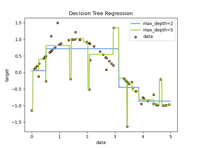
Example. Regression Trees of Different Depths
The more complex the tree (the greater its depth), the higher the influence of noise in the data and the higher the risk of overfitting.
CART: Minimal Cost-Complexity Pruning Criterion
Mean squared error with a penalty for tree complexity:
\[ C_\alpha(a) = \sum\limits_{i=1}^\ell (a(x_i) - y_i)^2 + \alpha |V_{\text{leaf}}| \to \min\limits_\alpha \]As \(\alpha\) increases, the tree is progressively simplified. Moreover, the sequence of nested trees is unique. From this sequence, the tree with the minimum error on the test sample (Hold-Out) is selected.
For the case of classification, a similar pruning strategy is used, but with the Gini criterion.
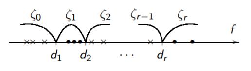
Auxiliary Task of Binarization of a Real Feature
Purpose: to reduce the enumeration of predicates of the form \([{\color{orange}\alpha} \leq f(x) \leq {\color{orange}\beta}]\)
Given: a set of real-valued feature vectors \(f(x_i), x_i \in X^l\)
Find: the best (in any sense) division of the feature value range into a relatively small number of zones:
- \(\zeta_0(x) = [f(x) < d_1]\)
- \(\zeta_s(x) = [d_s \leq f(x) < d_{s+1}], s = 1, \dots, r-1\)
- \(\zeta_r(x) = [d_r \leq f(x)]\)
Ways to Partition the Feature Value Area into Zones
- Greedy Information Maximization by Merging
- Division into Equally Powered Subsamples
- Partitioning by a Uniform Grid of "Convenient" Values
- Combining Several Partitions — for Example, Uniform and Median
Summary
- Basic requirements for logical regularities:
- interpretability
- informative
- diversity
- Advantages of decision trees:
- interpretability
- mixed types of data allowed
- capability to bypass missing data
- Drawbacks of decision trees:
- overfitting
- fragmentation
- instability to noise, composition of the sample, criteria
- Ways to eliminate these drawbacks:
- reduction
- regularization
- ensembles (forests) of trees — coming soon!