Machine learning with Python
Lecture 21. Bayesian methods intro
Alex Avdiushenko
December 19, 2023
Conditional Probability
$P(y|x) =\frac{P(x, y)}{P(x)}$
Example
The probability of rolling a 6 on a die given that an even number has rolled.
$P(6|\mathrm{even}) = \frac{P(\mathrm{even},\ 6)}{P(\mathrm{even})} = \frac13$
Symmetry: $$P(y|x)P(x) = P(x, y) = P(x|y)P(y)$$
Marginalization
\[ p(y|x)p(x) = p(x, y) = p(x|y)p(y) \Rightarrow \]
\[ \Rightarrow p(y|x) = \frac{p(x|y)p(y)}{p(x)} \]
\[ p(x) = \int p(x, y)dy = \int p(x|y)p(y)dy = E_y p(x|y)\]
Rules of Sum and Product
Sum Rule:
\[p(x_1, \dots , x_k) = \int p(x_1, \dots , x_k, \dots , x_n)d{x_{k+1}} \dots d{x_n}\]Product Rule:
\[ p(x_1, x_2, x_3, \dots , x_{n−1}, x_n) = p(x_1|x_2, x_3, \dots, x_{n−1}, x_n) \cdot \\ \cdot p(x_2|x_3, \dots, x_{n−1}, x_n) \cdot \ldots \cdot p(x_{n}) \]Bayes' Theorem
Example with a Friend and an Exam
Given:
- $x$ — student is (not) happy
- $y$ — exam is (not) passed
- $P(\text{exam is passed}) = 1/3$
- $P(\text{student is happy}|\text{exam is passed}) = 1$
- $P(\text{student is happy}|\text{exam is NOT passed}) = 1/6$
Find:
$P(y=1|x=1) = P(\mathrm{exam\ is\ passed}|\mathrm{student\ is\ happy})\ —\ ?$
Solution:
Graphical Models
$$p(x_1, x_2, x_3, x_4, x_5) = \\ p(x_1 | x_3) p(x_2 | x_4)p(x_3 | x_4, x_5)p(x_4)p(x_5)$$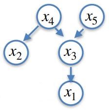
For example, what influences a friend's mood?

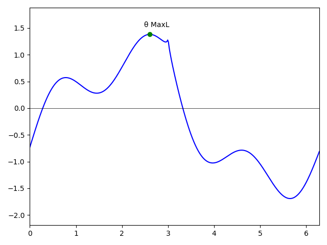
Maximum Likelihood Method (frequentist approach)
Properties of MaxL:
- MaxL estimate is consistent: $$\theta_{\text{MaxL}} \overset{p}{\to} \theta_{\text{ground truth}}$$
- Asymptotically efficient: there is no consistent estimate that improves mean-square error as $n \to \infty$
- Asymptotically normal: $$\sqrt{n} \left(\theta_{\text{MaxL}} - \theta_{\text{ground truth}}\right) \overset{d}{\to} N(0, \text{FI}^{-1})$$
Bayesian approach to the problem of machine learning
$$p(\theta|X) = \frac{p(X|\theta)p(\theta)}{\int p(X|\theta)p(\theta)d\theta}$$Comparison of Approaches
| $\quad\quad\quad\quad$ | Frequentist Approach (Fischer) | Bayesian Approach |
|---|
| Relationship to Randomness | Cannot predict | Can predict given enough information |
|---|
| Values $\quad\quad\quad$ | Random and deterministic | All random |
|---|
| Inference Method | Maximum likelihood | Bayes' Theorem |
|---|
| Parameter Estimates | Point estimates | Posterior distribution |
|---|
| Use Cases | $n \gg d$ | Always |
|---|
Relationship Between Frequentist and Bayesian Approaches
$$\lim\limits_{n \to \infty} p(\theta|x_1, \dots, x_n) = \delta(\theta - \theta_{\text{ML}})$$ $\delta$ — Dirac delta functionAdvantages of the Bayesian Approach
- Regularization
- Compositeness. For example, the popularity of topics on social networks — first, we calculated based on the news feed, then refined using video data
- On-the-fly data processing — iteratively update the posterior distribution
- We can calculate various statistics
- We can estimate the confidence in the values of model parameters
Confidence Estimation
Computational Difficulties
Calculation Methods
- Analytical calculation
- Markov chain Monte Carlo (MCMC)
- Variational inference (not covered in the first part of the course)
Analytical Approach (conjugate distributions)
Let $p(x|\theta) = A(\theta)$ and $p(\theta) = B(\alpha)$
The prior distribution of parameters $p(\theta)$ is called conjugate to $p(x|\theta)$ (conjugate priors), if the posterior distribution belongs to the same family as the prior $p(\theta|x) = B(\alpha^\prime)$
Knowing the formula for the family to which our posterior distribution should belong, it is easy to calculate its normalizing factor (the integral in the denominator)
Example 1
Posterior distribution of the expected value of a normal distribution
Normal distribution:
$N(x|\mu, \sigma) = \frac{1}{\sigma \sqrt{2\pi}} \exp\left(-\frac{(x-\mu)^2}{2\sigma^2} \right)$Likelihood:
$p(x|\mu) = N(x|\mu, 1) = \frac{1}{\sqrt{2\pi}} \exp\left(-\frac{(x-\mu)^2}{2} \right)$Conjugate prior:
$p(\mu) = N(\mu|m,s^2)$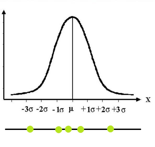
Example 2
Posterior probability of getting heads when flipping a biased coin
Frequentist approach
$q$ — the probability of heads equals the fraction of heads in $n$ flips
Likelihood
Binomial distribution: $p(x|q) = C_n^x q^x (1-q)^{n-x}$
Conjugate prior
Beta distribution: $p(q| \alpha, \beta) = \frac{q^{\alpha-1} (1-q)^{\beta-1}}{B(\alpha, \beta)}$
The numerator of the posterior distribution:
$$q^{\alpha-1+x} (1-q)^{\beta-1+(n-x)} = q^{\alpha^\prime-1} (1-q)^{\beta^\prime-1},$$where $\alpha^\prime = \alpha + x, \beta^\prime = \beta + n - x$, so essentially, we also know the denominator, it equals $B(\alpha^\prime, \beta^\prime)$.
Posterior distribution
$$p(q|x) = \frac{q^{\alpha-1+x} (1-q)^{\beta-1+(n-x)}}{B(\alpha + x, \beta + n - x)}$$Markov chain Monte Carlo
Motivation
- We'd like to be able to calculate mathematical expectations and other quantities according to the posterior distribution, known up to a constant
- For example, we'd like to know the response of an ensemble consisting of an infinite number of algorithms :)
- We can sum up (integrate) the expected responses of the classifier, according to the probability of the model parameters
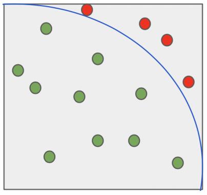
Monte Carlo Method
A broad class of computational algorithms based on the repeated execution of random experiments and the subsequent calculation of quantities of interest.
$$\int f(x)dx \approx \frac{1}{n} \sum\limits_{i=1}^n f(x_i)$$- Invented by Stanislaw Ulam in 1949 when he was playing solitaire while ill and wondered what is the probability of being able to play out all the cards? He didn't solve it combinatorically, but simply by the share of successful games
- The method was named after the Monte Carlo casino in Monaco for the sake of secrecy since it was used in the Manhattan Project for the development of nuclear weapons in the USA
Example of Using the Monte Carlo Method
Markov Chains
- Markov chains are used for modeling many probability distributions
- That is, it's possible to construct a process where the sequence $x$ will appear to have been generated from a probability distribution
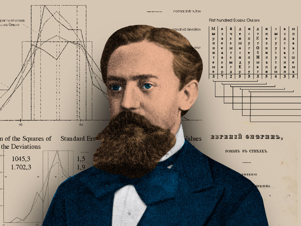
Andrey Andreyevich Markov (senior), 1906
The sequence $x_1, x_2, \dots, x_{n-1}, x_n$ is a Markov chain, if
$$p(x_1, x_2, \dots, x_{n-1}, x_n) = p(x_n|x_{n-1}) \dots p(x_2|x_1)p(x_1)$$
MCMC in Calculating Mathematical Expectations
In this case, we can use the Monte Carlo method to calculate mathematical expectations for this probability distribution
$$E_{p(x)} f(x) \approx \frac{1}{n} \sum\limits_{i=1}^n f(x_i),$$where $x_i \sim p(x)$
Gibbs Sampling (1984)
An instance of the Metropolis-Hastings algorithm, named after the distinguished scientist Josiah Gibbs.
Suppose we derived the posterior distribution only up to a normalization constant:
$$p(x_1, x_2, x_3) = \frac{\hat p(x_1, x_2, x_3)}{C}$$
Josiah Willard Gibbs
We start with $(x_1^0, x_2^0, x_3^0)$, and within a loop, we perform the following procedure:
- $x_1^1 \sim p(x_1 | x_2 = x_2^0, x_3 = x_3^0)$
- $x_2^1 \sim p(x_2 | x_1 = x_1^1, x_3 = x_3^0)$
- $x_3^1 \sim p(x_3 | x_1 = x_1^1, x_2 = x_2^1)$
- $x_1^2 \sim p(x_1 | x_2 = x_2^1, x_3 = x_3^1)$ etc.
After a few iterations "the chain has warmed up", we can estimate expectations based on these samples.
Sampling from a One-Dimensional Distribution
Rejection Sampling
\(i = 0\), repeat many times:
- sample \(y \sim q(y)\)
- sample \(\xi \sim U[0;Cq(y)]\)
- if \(\xi < \hat p(y)\):
- \(x_i = y\)
- \(i = i+1\)
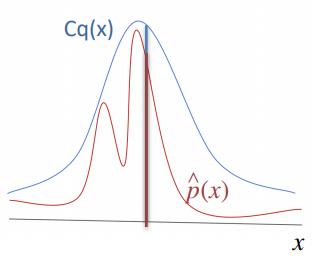
The difficulty lies in choosing the parameter \(C\), it's often too large.
Summary
- The frequentist approach is a limiting case of the Bayesian approach.
- The Bayesian approach has many nice properties:
- Regularization
- Composability
- Processing data "on the fly"
- Ability to calculate various statistics
- Ability to estimate confidence
- However, it is often computationally expensive.
- It is possible to use some advantages of the Bayesian approach without calculating the normalizing constant.