Youth AI club
Attention mechanism and Transformer architecture
Alex Avdiushenko
December 11, 2024
In the last episode
- Makemore on bigrams level
- Adding prior for more robust predictions
- Multi Layer Perceptron
Recurrent Neural Network scheme
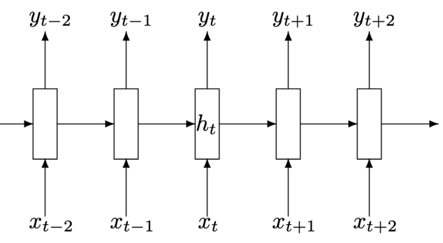
Disadvantages of vanilla Recurrent Neural Network (reminder)
We use one hidden vector
$$ h_t = f_W(h_{t-1}, x_t) $$As a function \(f_W\) we set a linear transformation with a non-linear component-wise "sigmoid":
$$ \begin{align*} h_t &= \tanh ({\color{orange}W_{hh}} h_{t-1} + {\color{orange}W_{xh}} x_t) \\ y_t &= {\color{orange}W_{hy}} h_t \end{align*} $$- Input and output sequence lengths must match
- "Reads" the input only from left to right, does not look ahead
- Therefore, it is not suitable for machine translation, question answering tasks, and others
RNN for sequence synthesis (seq2seq, reminder)
$X = (x_1, \dots, x_n)$ — input sequence
$Y = (y_1, \dots, y_m)$ — output sequence
\(\color{green}c \equiv h_n\) encodes all information about \(X\) to synthesize \(Y\)
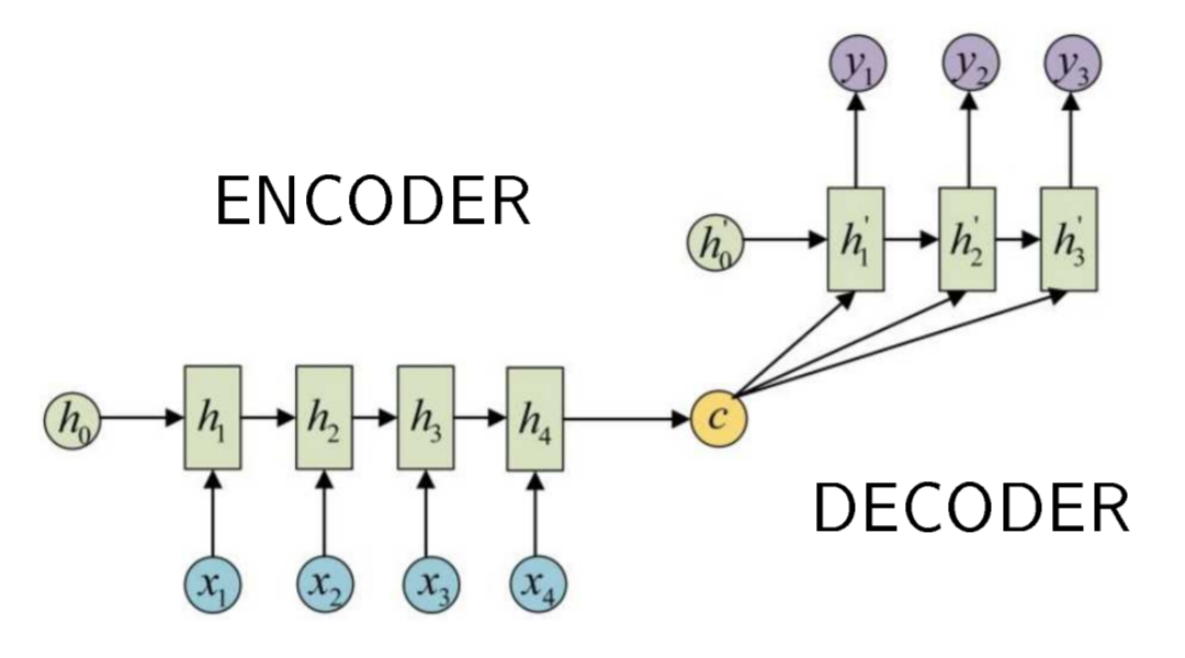
Disadvantages
- ${\color{green}c}$ remembers the end ($h_n$) better than the start
- The more $n$, the more difficult to pack all the information into vector ${\color{green}c}$
- We should control the vanishing and explosions of the gradient
- RNN is difficult to parallelize
Let's count the number of passes
RNN with an attention mechanism
\(a(h, h^\prime)\) is the similarity function of input \(h\) and output \(h^\prime\) (for example, dot product or \(\exp(h^T h^\prime)\) and others)
\(\alpha_{ti}\) — importance of input \(i\) for output \(t\) (attention score), \(\sum\limits_i \alpha_{ti} = 1\)
\(c_t\) — input context vector for output \(t\)
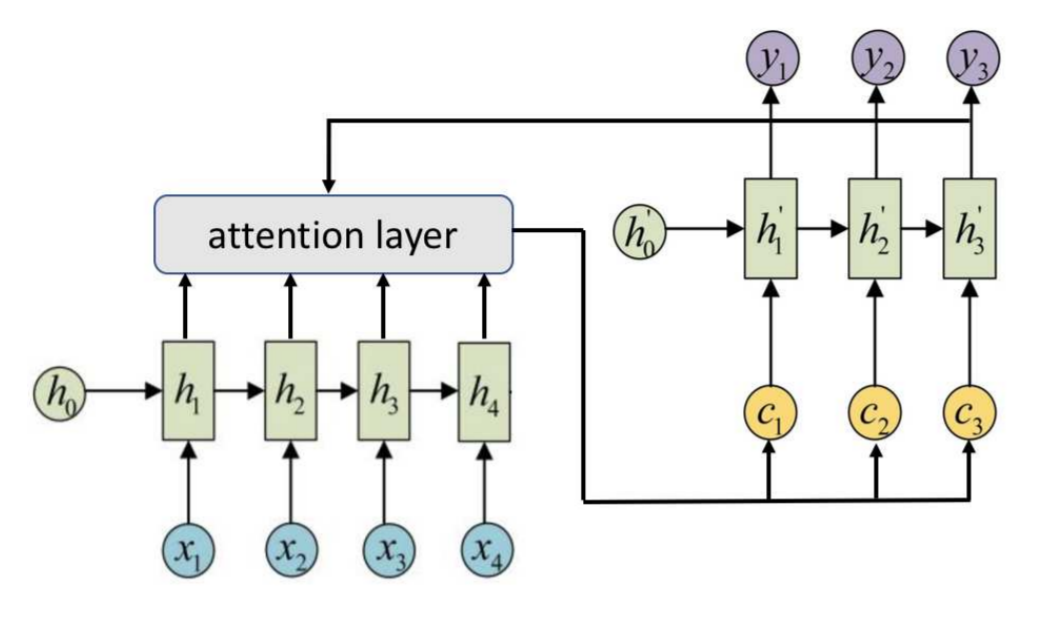
- You can enter trainable parameters in \({\color{green}\alpha}\) and \({\color{green}c_t}\)
- It is possible to refuse recurrence both in \(h_i\) and in \(h_t^\prime\)
Bahdanau et al. Neural machine translation by jointly learning to align and translate. 2015
The Main Areas for Attention Models
Converting one sequence to another, i.e. seq2seq:
- Machine translation
- Question answering
- Text summarization
- Annotation of images, videos (multimedia description)
- Speech recognition
- Speech synthesis
Sequence processing:
- Classification of text documents
- Document Sentiment Analysis
Attention in machine translation
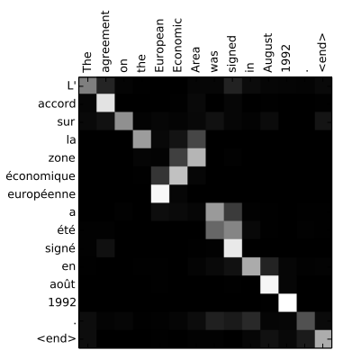
Attention Model Interpretability: Visualization of \(\alpha_{ti}\)
Attention for annotating images
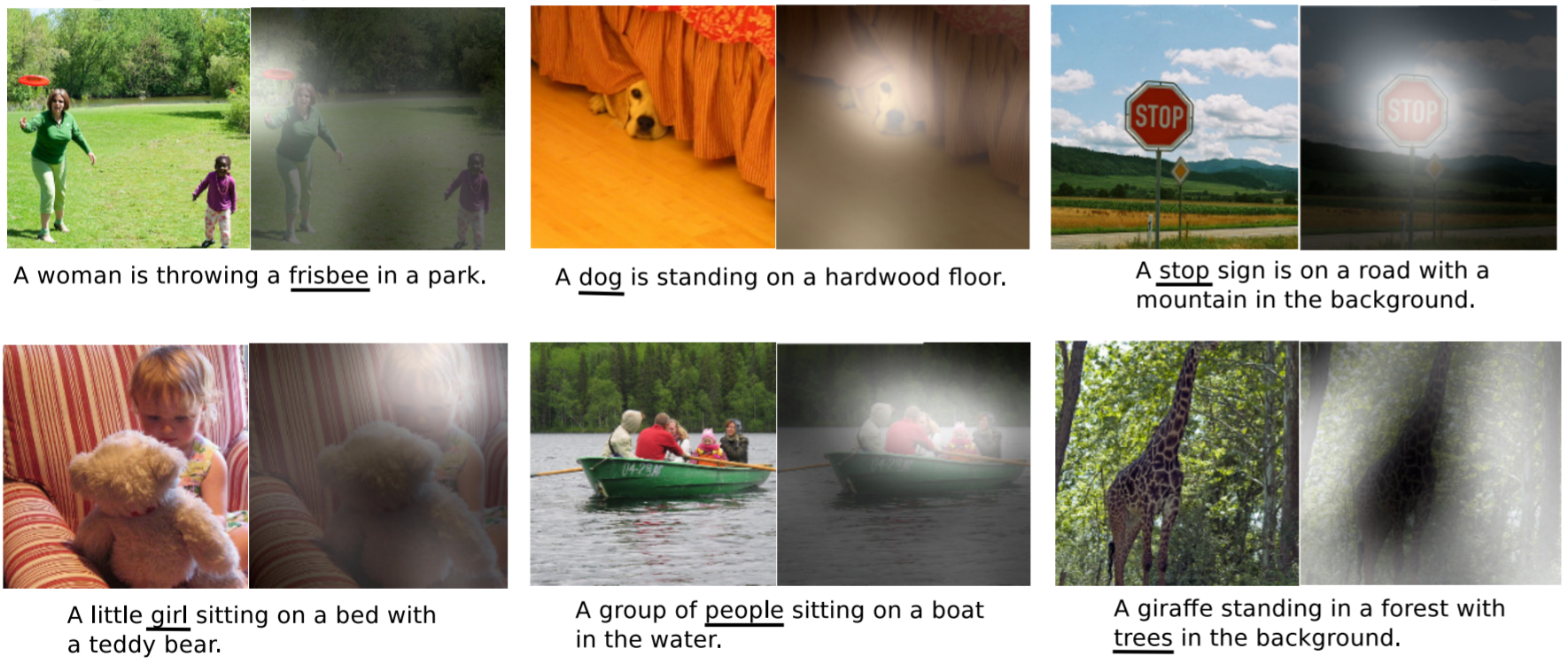
When generating a word for an image description, the visualization shows which areas of the image the model pays attention to
Vector Similarity Functions:
\(a(h, h^\prime) = h^T h^\prime\) is the scalar (inner) product
\(a(h, h^\prime) = \exp(h^T h^\prime)\) — with
norm becomes SoftMax
\(a(h, h^\prime) = h^T {\color{orange}W} h^\prime\) — with the learning parameter matrix \(\color{orange}{W}\)
\(a(h, h^\prime) = {\color{orange}w^T} \tanh ({\color{orange}U}h + {\color{orange}V} h^\prime)\) is additive attention with \({\color{orange}w, U, V}\)
Linear vector transformations: query, key, value
\(a(h_i, h^\prime_{t-1}) = ({\color{orange}W_k}h_i)^T ({\color{orange}W_q}h^\prime_{t-1}) / \sqrt{d}\)
\(\alpha_{ti} = \text{SoftMax}_i a(h_i, h^\prime_{t-1})\)
\(c_t = \sum\limits_i \alpha_{ti} {\color{orange}W_v} h_i\)
\({\color{orange}W_q}_{d \times dim(h^\prime)}, {\color{orange}W_k}_{d \times dim(h)}, {\color{orange}W_v} _{d \times dim(h)}\) — linear neuron weight matrices,
possible simplification: \({\color{orange}W_k} \equiv {\color{orange}W_v}\)
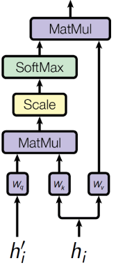
Attention Formula
\(q\) is the query vector for which we want to calculate the context
\(K = (k_1, \dots, k_n)\) — key vectors compared with the query
\(V = (v_1, \dots, v_n)\) — value vectors forming the context
\(a(k_i, q)\) — score of relevance (similarity) of key \(k_i\) to query \(q\)
\(c\) is the desired context vector relevant to the query
This is a 3-layer network that computes a convex combination of \(v_i\) values relevant to the query \(q\):
\[ c = \text{Attn}(q,K,V) = \sum\limits_i v_i \, \text{SoftMax}_i \, a(k_i, q) \]\(c_t = \text{Attn}({\color{orange}W_q} h^\prime_{t-1}, {\color{orange}W_k} H, {\color{orange}W_v} H)\) is the example from the previous slide, where \(H = (h_1, \dots, h_n)\) comes from encoder, \(h^\prime_{t-1}\) comes from decoder
Self-attention:
\(c_i = \text{Attn}({\color{orange}W_q} h_{i}, {\color{orange}W_k} H, {\color{orange}W_v} H)\) is a special case when \(h^\prime \in H\)
Multi-Head Attention
Idea: \(J\) different attention models are jointly trained to highlight various aspects of the input information (for example, parts of speech, syntax, idioms):
\( c^j = \text{Attn}({\color{orange}W^j_q} q, {\color{orange}W^j_k} H, {\color{orange}W^j_v} H), j = 1, \dots, J\)
Variants of aggregating the output vector:
- \( c = \frac{1}{J} \sum\limits_{j=1}^J c^j\) — averaging
- \( c = [c^1 \dots c^J]\) — concatenation
- \( c = [c^1 \dots c^J] {\color{orange}W}\) — to return to the desired dimension
Transformer for Machine Translation
It is a neural network architecture based on attention and fully connected layers, without RNN. Scheme of transformations in machine translation:
- \(S = (w_1, \dots, w_n)\) — sentence from words in the input language
- \(X = (x_1, \dots, x_n)\) — embeddings of input sentence words
- \(Z = (z_1, \dots, z_n)\) — contextual embeddings
- \(Y = (y_1, \dots, y_m)\) — embeddings of output sentence words
- \(\tilde S = (\tilde w_1, \dots, \tilde w_m)\) — sentence words in target language
\(\downarrow\) trainable or pre-trained word vectorization \(\downarrow\)
\(\downarrow\) encoder \(\downarrow\)
\(\downarrow\) decoder \(\downarrow\)
\(\downarrow\) generation of words from the constructed language model \(\downarrow\)
Architecture of Transformer: Encoder
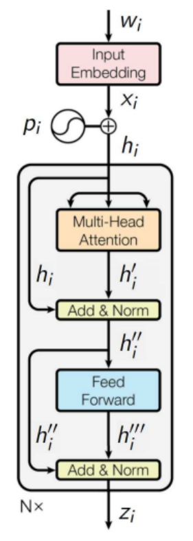
- Position vectors \(p_i\) are added:
\(h_i = x_i + p_i, \ H = (h_1, \dots, h_n)\) \(\scriptscriptstyle d = \text{dim } x_i, p_i, h_i = 512\)
\(\scriptscriptstyle \text{dim } H = 512 \times n\) - Multi-head self-attention:
\(h_i^j = \text{Attn}({\color{orange}W_q^j} h_{i}, {\color{orange} W_k^j} H, {\color{orange}W_v^j} H)\) \(\scriptscriptstyle j = 1, \dots, J = 8\)
\(\scriptscriptstyle \text{dim } h_i^j = 64\)
\(\scriptscriptstyle \text{dim } W_q^j, W_k^j, W_v^j = 64 \times 512\) - Concatenation:
\(h_i^\prime = MH_j(h_i^j) \equiv [h_i^1 \dots h_i^J]\) \(\scriptscriptstyle \text{dim } h_i^\prime = 512\) - Skip-connection and layer normalization:
\(h_i^{\prime\prime} = LN(h_i^\prime + h_i; {\color{orange}\mu_1, \sigma_1})\) \(\scriptscriptstyle \text{dim } h_i^{\prime\prime}, \mu_1, \sigma_1 = 512\)
Architecture of Transformer: Encoder

- Fully connected two-layer network FFN:
\(h_i^{\prime\prime\prime} = {\color{orange} W_2} \text{ReLU}({\color{orange} W_1}h_i^{\prime\prime} + {\color{orange} b_1}) + {\color{orange} b_2}\) \(\scriptscriptstyle \text{dim } W_1 = 2048 \times 512\)
\(\scriptscriptstyle \text{dim } W_2 = 512 \times 2048\) - Skip-connection and layer normalization:
\(z_i = LN(h_i^{\prime\prime\prime} + h_i^{\prime\prime}; {\color{orange}\mu_2, \sigma_2})\) \(\scriptscriptstyle \text{dim } z_i, \mu_2, \sigma_2 = 512\)
Additions and Remarks
- A lot of such blocks \(N=6, h_i \to \square \to z_i\) are connected in series
- Calculations can be easily parallelized in \(x_i\)
- It is possible to use pre-trained \(x_i\) embeddings
- It is possible to learn embeddings \(x_i\) of words \(w_i \in V\)
- Layer Normalization (LN), \(x, {\color{orange}\mu}, {\color{orange}\sigma} \in \mathbb{R}^d\):
Positional Encoding
The positions of the words \(i\) are encoded by the vectors \(p_i\) so that:
- The more \(|i-j|\), the more \(\|p_i-p_j\|\)
- The number of positions is not limited
For example,
\[ h_j = \text{Attn}(q_j, K, V) = \sum_i (v_i + {\color{orange}w^v_{i\boxminus j}}) \text{SoftMax}_i a(k_i + {\color{orange} w^k_{i\boxminus j}}, q_j), \]where \(i\boxminus j = \max(\min(i-j, \delta), -\delta)\) is the truncated difference, \(\delta = 5..16\)
Architecture of Transformer: Decoder
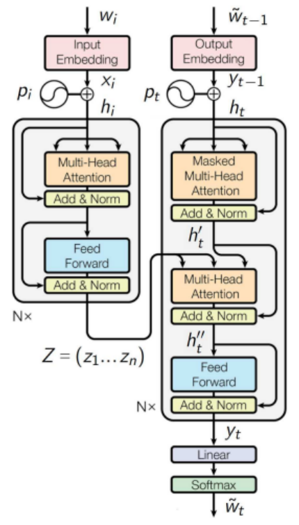
Autoregressive sequence synthesis
\(y_0 = \left< \text{BOS} \right>\) — start symbol embedding;
For all \(t = 1, 2, \dots\)
- Masking data "from the future":
\(h_t = y_{t-1} + p_t; \ H_t = (h_1, \dots, h_t)\)
- Multi-head self-attention:
\(h_t^\prime = {\color{olive} LN_{sc}} \circ MH_j \circ \text{Attn}({\color{orange}W_q^j} h_{t}, {\color{orange} W_k^j} H_t, {\color{orange}W_v^j} H_t)\)
- Multi-head attention on the Z vectors:
\(h_t^{\prime\prime} = {\color{olive} LN_{sc}} \circ MH_j \circ \text{Attn}({\color{orange}\tilde W_q^j} h_{t}^\prime, {\color{orange}\tilde W_k^j} Z, {\color{orange}\tilde W_v^j} Z)\)
Architecture of Transformer Decoder

- Two-layer neural network:
\(y_t = {\color{olive} LN_{sc}} \circ \text{FFN}(h_t^{\prime\prime})\)
- Linear predictive layer:
\(p(\tilde w|t) = \text{SoftMax}_{\tilde w}({\color{orange} W_y} y_t + {\color{orange} b_y})\)
- Generation \(\tilde w_t = \arg\max\limits_{\tilde w} p(\tilde w|t)\)
until \(\tilde w_t \neq \left< \text{EOS} \right>\)
Training and Validation Criteria for Machine Translation
Criteria for learning parameters of the neural network \({\color{orange}{W}}\) on the training set of sentences \(S\) with translation \(\tilde S\):
$$ \sum\limits_{(S, \tilde S)} \sum\limits_{\tilde w_t \in \tilde S} \ln p(\tilde w_t|t, S, {\color{orange}W}) \to \max\limits_W $$Criteria for evaluating models (non-differentiable) based on a sample of pairs of sentences "translation \(S\), standard \(S_0\)":
BiLingual Evaluation Understudy:
\(\text{BLEU} = \text{Brevity Penalty} \times \text{n-gram overlap}
= \min \left(1, \frac{ \text{len}(S)}{\text{len}(S_0)} \right) \times \)
\(\underset{(S_0, S)}{\text{mean}}\left(\prod\limits_{n=1}^4 \frac{\#n\text{-gram from } S, \text{incoming in } S_0}{\#n\text{-gram in } S} \right)^{\frac14}\)
BERT — Bidirectional Encoder Representations from Transformers
The BERT transformer is a decoderless encoder that can be trained to solve a wide range of NLP problems. Scheme of data transformations in NLP tasks:
- \(S = (w_1, \dots, w_n)\) — sentence from words in the input language
- \(X = (x_1, \dots, x_n)\) — embeddings of input sentence words
- \(Z = (z_1, \dots, z_n)\) — contextual embeddings
- \(Y\) — output text / markup / classification, etc.
\(\downarrow\) learning embeddings with transformer \(\downarrow\)
\(\downarrow\) encoder transformer \(\downarrow\)
\(\downarrow\) additional training for a specific task \(\downarrow\)
BERT: pre-training of deep bidirectional transformers for language understanding. 2019
MLM (Masked Language Modeling) Criterion for BERT Training
The masked language modeling criterion is built automatically from texts (self-supervised learning):
$$ \sum\limits_{S} \sum\limits_{ i \in M(S)} \ln p(w_i|i, S, {\color{orange}W}) \to \max\limits_W, $$where \(M(S)\) is a subset of masked tokens from \(S\),
$$ p(w|i, S, {\color{orange}W}) = \underset{w \in V}{\text{SoftMax}}({\color{orange}W_z}z_i(S, {\color{orange}W_T}) + {\color{orange}b_z})$$is a language model that predicts the \(i\)-th sentence token \(S\), \(z_i(S, {\color{orange}W_T})\) is the contextual embedding of the \(i\)-th sentence token \(S\) at the output of the transformer with parameters \({\color{orange}W_T}\), \({\color{orange}W}\) — all transformer and language model parameters
A Few More Notes About Transformers
- Fine-tuning: model \(f(Z(S, {\color{orange}W_T}), {\color{orange}W_f})\), sample \(\{S\}\) and criterion \(\mathcal{L}(S, f) \to \max\)
- Multitask learning: for additional training on a set of tasks \(\{t\}\), models \(f_t(Z(S, {\color{orange}W_T}), {\color{orange}W_f})\), samples \(\{S\}_t\) and sum of criteria \( \sum_t \lambda_t \sum_S \mathcal{L}_t(S, f_t) \to \max \)
- GLUE, SuperGLUE — sets of test problems for understanding natural language
- Transformers are usually built not on words, but on tokens received by BPE (Byte-Pair Encoding) or SentencePiece
- First transformer: \(N = 6, d = 512, J = 8\), weights 65M
- \(\text{BERT}_{\text{BASE}}\), GPT-1: \(N = 12, d = 768, J = 12\), weights 110M
- \(\text{BERT}_{\text{LARGE}}\), GPT-2: \(N = 24, d = 1024, J = 16\), weights 340M-1000M
- GPT-3: weights 175 billion
- Gopher (DeepMind): 280 billion
- Turing-Megatron (Microsoft + Nvidia): 530 billion
Summary
- Attention models were first built into RNNs or CNNs, but they turned out to be self-sufficient
- Based on them, the Transformer architecture was developed, various variants of which (BERT, GPT, XLNet, ELECTRA, etc.) are currently SotA in natural language processing tasks, and not only
- Multi-head self-attention (MHSA) has been proven to be equivalent to a convolutional network [Cordonnier, 2020]
Dichao Hu. An Introductory Survey on Attention Mechanisms in NLP Problems. 2018.
Xipeng Qiu et al. Pre-trained models for natural language processing: A survey. 2020.
Cordonnier et al. On the relationship between self-attention and convolutional layers. 2020.
What Else Can You Look at?
- GPT-3 on Wikipedia: https://en.wikipedia.org/wiki/GPT-3
- Intro to LLMs by Andrej Karpathy, November 2023
Regularization: to make aspects of attention as different as possible, rows \(J \times n\) of matrices \(A, \alpha_{ji} = \text{SoftMax}_i a({\color{orange}W_k^j}h_i, {\color{orange}W_q^j}q)\), decorrelated \((\alpha_{s}^T\alpha_{j} \to 0)\) and sparse \((\alpha_{j}^T\alpha_{j} \to 1)\):
\(\|AA^T - I \|^2 \to \min\limits_{\{{\color{orange}W_k^j}, {\color{orange}W_q^j}\}} \)
NSP (Next Sentence Prediction) Criterion for BERT Training
The criterion for predicting the relationship between NSP sentences is built automatically from texts (self-supervised learning):
$$ \sum\limits_{(S, S^\prime)} \ln p\left(y_{SS^\prime}|S, S^\prime, {\color{orange}W}\right) \to \max\limits_W, $$where \(y_{SS^\prime} = \) \(\left[S\right.\) followed by \(\left.S^\prime\right]\) is the binary classification of a pair of sentences,
$$ p(y|S, S^\prime, {\color{orange}W}) = \underset{y \in \{0,1\}}{\text{SoftMax}}\left({\color {orange}W_y} \tanh({\color{orange}W_s}z_0(S, S^\prime, {\color{orange}W_T}) + {\color{orange}b_s}) + {\color{orange}b_y}\right)$$— probabilistic classification model for pairs \((S, S^\prime)\), \(z_0(S, S^\prime, {\color{orange}W_T})\) — contextual embedding of token \(\left<\text{CLS}\right>\) for a sentence pair written as \(\left<\text{CLS}\right> S \left<\text{SEP}\right> S^\prime \left<\text{SEP}\right>\)