Reinforcement learning intro

Advanced machine learning

Reinforcement learning intro

Alex Avdiushenko
March 19, 2024

Problem Statement

Up to this point, we either restored the function from the training set $(X, Y)$ (supervised learning) or searched for the structure in the set of objects $X$ (unsupervised learning)
But how does learning work in the real world? Usually we do some action and get the result, gradually learning

Good morning, dear students. Today we are going to talk about reinforcement learning, it is a slightly separate topic that is not directly related to deep learning, but is included in machine learning. It is quite possible to read a semester course on it, but we will limit ourselves to a couple of lectures. Great, let's go on and let me remind you, that up to this point, we found the appropriate function $f$, based on the training set. And it is called supervised learning. Or also we found the inner structure in the set of objects, you know, texts or images, and it is called unsupervised learning, when we haven't answers $y$. A pretty good illustration of reinforcement learning comes from the amazing ability of children to learn to walk. Initially they have muscles and mostly lie down and sleep. There are no any datasets for supervised or unsupervised learning, but the whole real physical world is around. Then they begin to roll over from their stomach to their back and back, then they learn to crawl, sit, stand, and finally, walk and run.

Real world

Deep Reinforcement Learning in Pacman

One more motivation

For example, we need to select the main page of a pizzeria website to attract the clients

Two fundamental difficulties in RL

Exploration vs. Exploitation
Credit assignment

What approaches are there?

Multi-armed bandits — a special case of reinforcement learning with only one state, i.e., without credit assignment difficulty

Also, there is a statistics approach (i.e. not RL): A/B testing — many users see potentially bad options; another problem is that in reality the group size should depend on the true probability values (e.g., conversions) which you don't know

Bernoulli's one-armed bandit

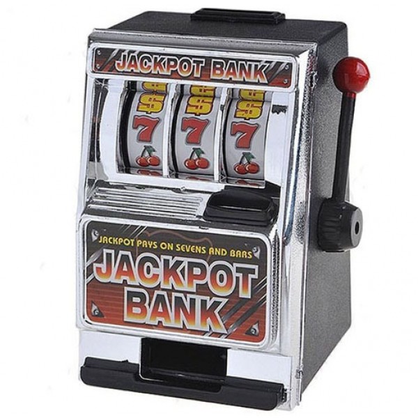
Probability of winning $\theta = 0.05$

Multi-Armed Bandits

$\theta_1 = 0.02$

$\theta_2 = 0.01 (min)$

$\theta_3 = 0.05$

$\theta_4 = 0.1 (max)$

We do not know the true probabilities, but we want to come up with a strategy that maximizes the payoff (reward)

Mathematical statement of the problem

Given possible actions $x_1, \dots, x_n$

At the next iteration $t$, for each action $x^t_i$ performed, we get the answer

$$ y^t_i \sim q(y|x^t_i, \Theta),$$

which brings us a reward

$$r_i^t = r(y^t_i)$$

There is an optimal action $x_{i^*}$ (sometimes $x_{i^*_t}$)

$$\forall i:\ \mathbb{E}(r_{i^*_t}^t) \geq \mathbb{E}(r^t_i) $$

Question: How to evaluate different strategies?

Measure of quality

The quality measure of the multi-armed bandit algorithm $a$ is usually regret

$$ R(a) = \sum\limits_{t=1}^T \left(\mathbb{E}(r_{i^*_t}^t) - \mathbb{E}(r_{i^a_t}^t)\right)$$

Under synthetic conditions (when we know the probabilities), we can consider

$$ E\left( R \right) = \int\limits_{\Theta} R(a)d\Theta $$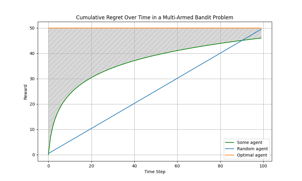

Multi-Armed Bandits possible applications

Areas:

advertising banners
recommendations (goods, music, movies etc.)
real slot machines in the casino

Approaches:

Thompson sampling
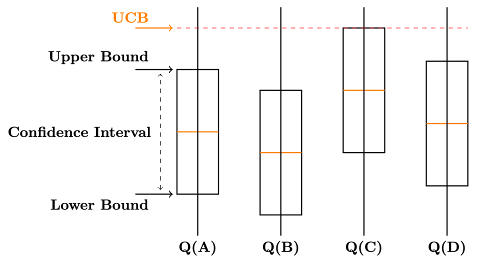
Upper Confidence Bound (UCB)
$\varepsilon$-greedy strategy

Multi-Armed Bandits Disadvantage

Do not take into account delayed effects. For example, the effect of clickbait in advertising

SHOCK! Cats want to enslave us

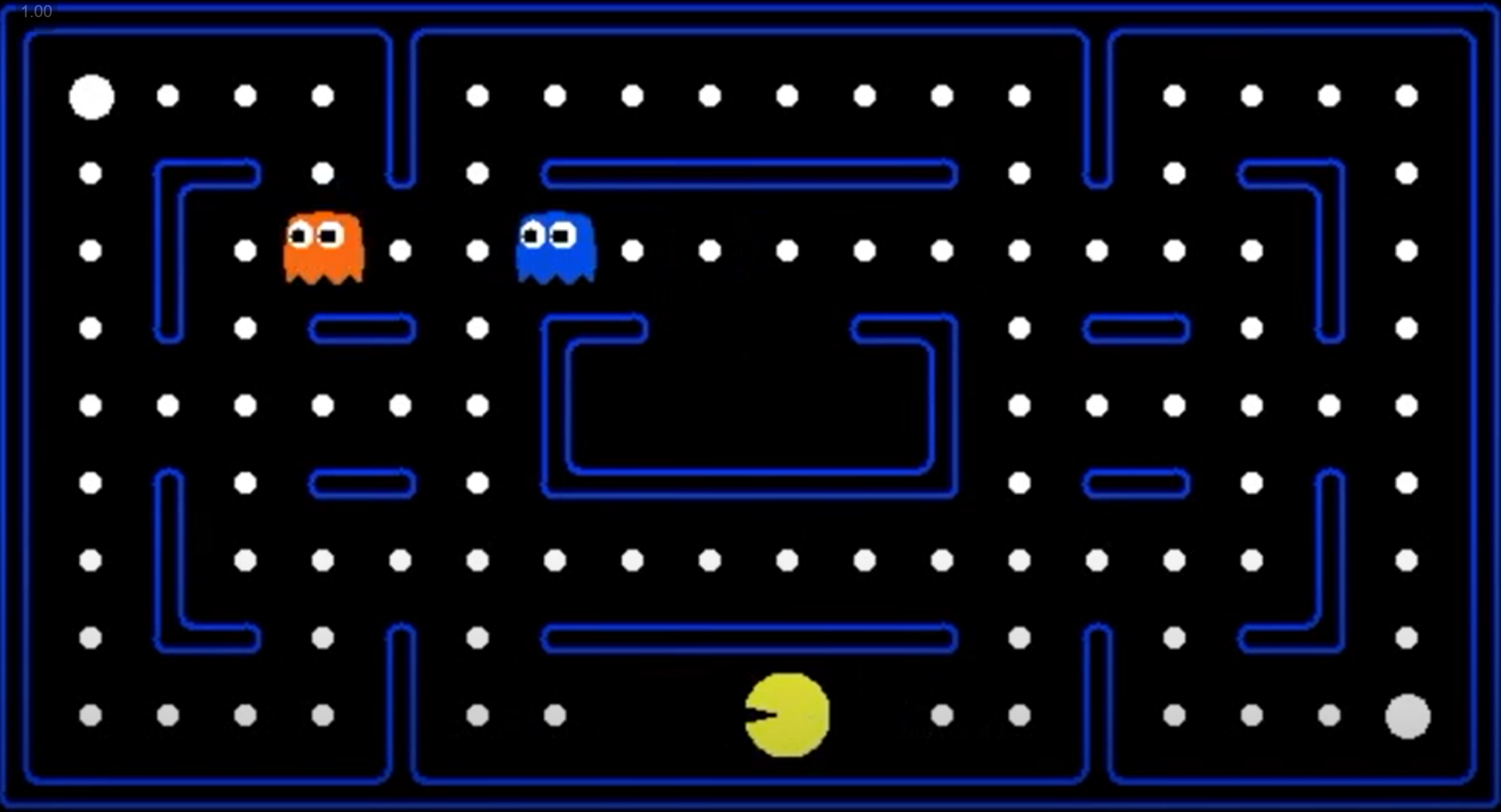
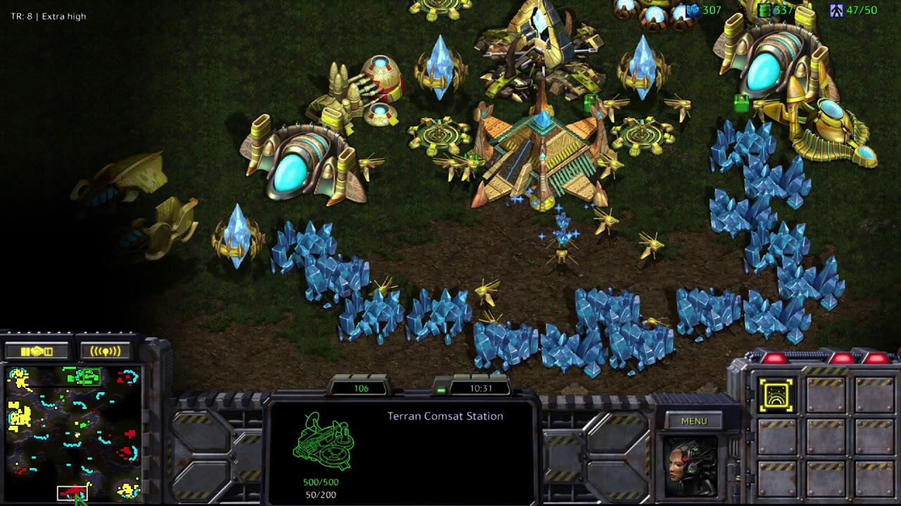
Reinforcement Learning Examples

robot control
(video) games
security management

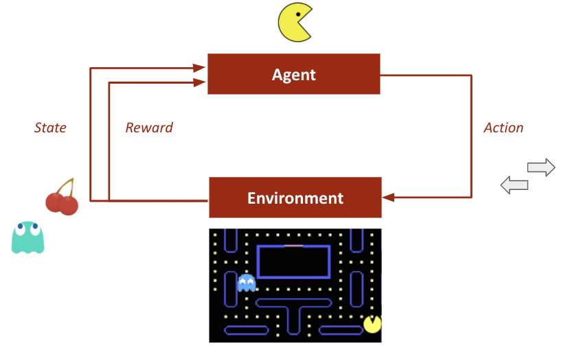
Agent Model in a Changing Environment

Definitions:

state $s \in S$
agent action $a \in A$
reward $r \in R$
state transition dynamics $P(s_{t+1} | s_t, a_t, \dots, s_{t-i}, a_{t-i}, \dots, s_0, a_0)$
win function $$r_t = r(s_t, a_t, \dots, s_0, a_0)$$
total reward $R = \sum\limits_t r_t$
agent policy $\pi (a | s)$

Task:

$$ \pi (a | s): \mathbb{E}_\pi [R] \to \max $$

Cross-entropy method. Algorithm

Trajectory — $[s_0, a_0, s_1, a_1, s_2, \dots, a_{T-1}, s_T]$

Initialize strategy model $\pi(a | s)$
Repeat:
- play $N$ sessions
- choose the best $K$ of them and take their trajectories
- adjust $\pi(a | s)$ so that strategy is able to maximize the probabilities of actions from the best trajectories

Cross-entropy method. Implementation with a table

As a strategy model, we simply take a matrix $\pi$ of dimension $|S| \times |A|$

$$\pi(a | s) = \pi_{s,a}$$

after selecting the best trajectories, we obtain a set of pairs

$$\text{Elite} = [(s_0, a_0), (s_1, a_1), (s_2, a_2), \dots, (s_H, a_H)]$$

and maximize the likelihood

$$ \pi_{s,a} = \frac{\sum\limits_{s_t, a_t \in \text{Elite}} [s_t = s][a_t = a]}{\sum\limits_{s_t, a_t \in \text{Elite}} [s_t = s]}$$

Training Example

There is a problem..

That there are a lot of states:

Approximate cross-entropy methods

Possible solutions:

Split the state space into sections and treat them as states
Get probabilities from $\pi_\theta (a | s)$ machine learning model: linear model, neural network, random forest (often these probabilities need to be further specified later)

Example

As a strategy model, we take just a neural network $\pi_\theta$
Initialize with random weights
At each iteration, after selecting the best trajectories, we obtain a set of pairs $$\text{Elite} = [(s_0, a_0), (s_1, a_1), (s_2, a_2), \dots, (s_H, a_H )]$$
And perform optimization $$ \pi = \arg\max\limits_\theta \sum\limits_{s_i, a_i \in \text{Elite}} \log \pi(a_i|s_i) = \arg\max\limits_\theta \mathscr{ L}(\theta)$$
That is $$ \theta_{t+1} = \theta_{t} + \alpha \nabla \mathscr{L}(\theta) $$

Disadvantages of the cross-entropy method

It is unstable for small samples
In the case of a non-deterministic environment, it chooses lucky cases (randomly played in favor of the agent)
It is focusing on behavior in simple states
It ignores a lot of information
There are tasks in which the end never comes (stock market game, for instance)

Markov Decision Process

Definitions:

state $s \in S$
agent action $a \in A$
reward $r \in R$
transition dynamics (Markov's assumption) $$ P(s_{t+1} | s_t, a_t, \dots, s_{t-i}, a_{t-i}, \dots, s_0, a_0) = P(s_{t+1} | s_t, a_t)$$
win function (Markov's assumption) $$r_{t} = r(s_t, a_t)$$
total reward $R = \sum\limits_t r_t$

Task:

agent policy $ \pi (a | s) $

$$ \pi (a | s): \mathbb{E}_\pi [R] \to \max $$

Important definitions

Average absolute win: $$ \mathbb{E}_{s_0 \sim P(s_0)\,} \mathbb{E}_{a_0 \sim \pi(a|s_0)\,} \mathbb{E}_{s_1, r_0 \sim P(s^\prime,r|s, a)} \dots \left[r_0 + r_1 + \dots + r_T \right]$$

On-Policy Value Function: $$ V_{\pi} (s) = \mathbb{E}_\pi [R_t|s_t = s] = \mathbb{E}_\pi \left[\sum\limits_{k=0}^\infty \gamma^k r_{k+t+1} | s_t = s\right]$$

On-Policy Action-Value Function: $$ Q_{\pi} (s, a) = \mathbb{E}_\pi [R_t|s_t = s, a_t = a] = \mathbb{E}_\pi \left[\sum\limits_{k=0}^\infty \gamma^k r_{k+t+1} | s_t = s, a_t = a \right]$$

where $\pi$ is the strategy followed by the agent, $\gamma \in [0, 1]$

Question: What is the meaning of the difference $Q_{\pi} (s, a) - V_{\pi} (s)$?

Often in RL, we don't need to describe how good an action is in an absolute sense, but only how much better it is than others on average. We make this concept precise with the advantage function: $$ A_{\pi} (s, a) = Q_{\pi} (s, a) - V_{\pi} (s) $$

Bellman Equation

For the Action-Value function $Q$

$$ Q_{\pi} (s,a) = \mathbb{E}_\pi \left[r_t + \gamma \sum\limits_{a^\prime} \pi(a^\prime|s^\prime) Q_{\pi}(s^\prime,a^\prime) \mid s_t = s, a_t = a \right]$$

State utility recalculation

$$V(s) = \max\limits_a [r(s, a) + \gamma V(s^\prime (s, a))]$$

That is, with probabilistic transitions

$$V(s) = \max\limits_a [r(s, a) + \gamma \mathbb{E}_{s^\prime \sim P(s^\prime | s, a)} V(s^ \prime)]$$

Iterative State Utility Recalculation Formula:

$$ \begin{align*} \forall s \ V_0(s) &= 0 \\ V_{i+1}(s) &= \max\limits_a [r(s, a) + \gamma \mathbb{E}_{s^\prime \sim P(s^\prime | s, a)} V_{i}(s^\prime)] \end{align*} $$

Note: To use this formula in practice, we need to know the transition probabilities $P(s^\prime| s, a)$

Utility of an action

$$Q(s, a) = r(s, a) + \gamma V(s^\prime)$$

The strategy of the game is defined as follows

$$\pi(s) : \arg\max\limits_a Q(s, a)$$

Again due to stochasticity

$$Q(s, a) = \mathbb{E}_{s^\prime} [r(s, a) + \gamma V(s^\prime)]$$

It is possible to estimate the expected value without an explicit distribution, using the Monte Carlo method and averaging over the outcomes:

$$Q(s_t, a_t) \leftarrow \alpha \left(r_t+\gamma \max\limits_a Q(s_{t+1}, a) \right) + (1-\alpha) Q(s_{t}, a_{t})$$

In theory, we can solve SLAE of Bellman Equations, get $Q^*(s,a)$ and that's it.

In practice, we have lots of problems:

how to enumerate all possible strategies $\pi$?
usually we don't know $r_t$ and probability distributions to calculate expectation
also, the amount of all state is really huge and uncountable

Let's consider optimal value function:

$$Q^*(s,a) = \max\limits_\pi \mathbb{E}_\pi [R_t|s_t = s, a_t = a] $$

We have similar Bellman Equation for $Q^*(s,a)$ and if we solved it, our strategy would be obvious: $$\pi^*(s) = \arg\max\limits_a Q^*(s,a)$$

$\quad$ The greedy strategy $\pi$ with respect to a solution of Bellman Equations $Q^*(s,a)$ (SLAE) "choose the action that maximizes $Q^*$" is optimal.

Temporal Difference training (TD)

$$ V_{\pi} (s) = \mathbb{E}_\pi [R_t|s_t = s] = \mathbb{E}_\pi \left[r_{t+1} + \gamma R_{t+1} | s_t = s\right] \\ \Rightarrow V_{\pi} (s_t) \sim R_{t+1} + \gamma V_{\pi} (s_{t+1}) $$

We arbitrarily initialise the function $V_{\pi}(s)$ and the strategy $\pi$. Then we repeat:

Initialise $s$
For each agent step:
- Select $a$ by strategy $\pi$
- Do action $a$, get result $r$ and next state $s^\prime$
- Update function $V(s)$ by formula $V(s) = V(s) + \alpha \left[r + \gamma V(s^\prime) - V(s)\right]$
- Go to the next step by assigning $s := s^\prime$

SARSA and Q-Learning in Temporal Difference (TD) Training

SARSA

State-Action-Reward-State-Action computes the Q-value based on the current state of the policy and is considered as an on-policy learning algorithm. Named by the quintuple (s,a,r,s',a'), the formula is as follows:

$$ Q(s,a) \leftarrow Q(s,a) + \alpha \left[r + \gamma Q(s',a') - Q(s,a)\right] $$

Q-Learning

Q-Learning is an off-policy learning algorithm that computes the Q-value based on the maximum reward that is attainable in the next state. The formula is as follows:

$$ Q(s,a) \leftarrow Q(s,a) + \alpha \left[r + \gamma \max_{a}\left[Q(s',a')\right] - Q(s,a)\right] $$

DQN (Deep Q-Learning Network)

Environment is Atari game emulator, and each frame is $210\times 160\text{ pix}, \ 128\text{ colors}$

Atari Games

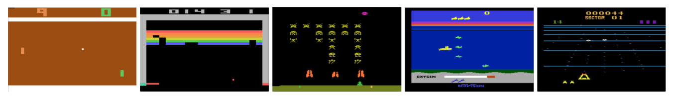
Pong

Breakout

Space Invaders

Seaquest

Beam Rider

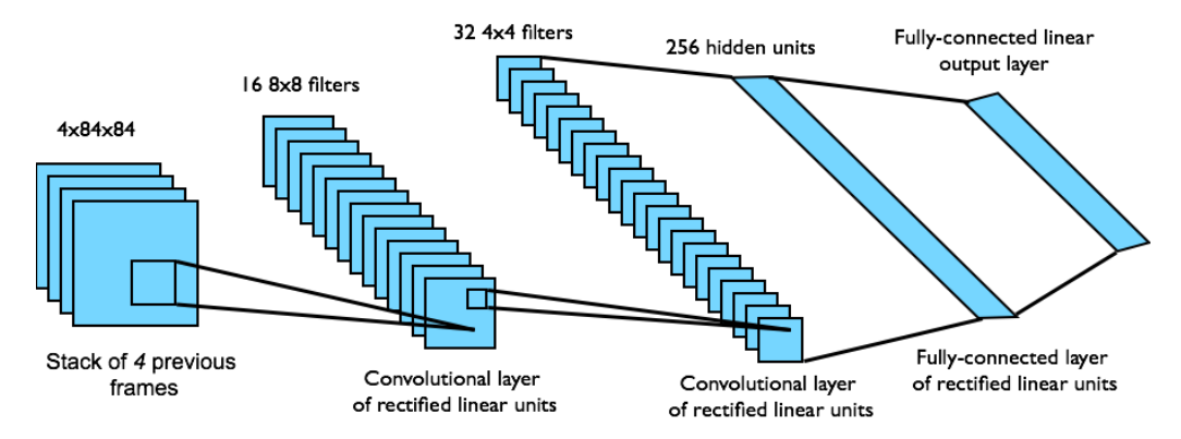
States s: 4 consecutive frames compressed to $84 \times 84$
Actions a: from 4 to 18, depending on the game
Rewards r: current in-game SCORE
Value function $Q(s, a; w)$: ConvNN with input $s$ and $|A|$ outputs

Source: V.Mnih et al. (DeepMind). Playing Atari with deep reinforcement learning. 2013

DQN Method

Saves trajectories $(s_t, a_t, r_t)_{t=1}^T$ in replay memory for repeated experience replay. It is needed to prevent overfitting
Gets approximation of the optimal value function $Q(s_t, a_t)$ for fixed current network parameters ${\color{orange} w_t}$
Evaluates loss function for training the neural network model $Q(s, a; w)$: $$ \mathscr{L} (w) = (Q(s_t, a_t; w) - y_t)^2 $$ with stochastic gradient SGD (by mini-batches of length 32): $$ w_{t+1} = w_{t} - \eta \left(Q(s_t, a_t; w_t) - y_t\right) \nabla_w Q(s_t, a_t; w_t) $$
Also it is better to use two different models for max evaluation and updating (Double Q-learnig by Hado van Hasselt, 2010)

Network architecture for the value function

DQL CNN Architecture

Dueling Networks

Dueling Network is a reinforcement learning architecture. The idea behind Dueling Networks is that in many settings, it could be beneficial to separate the representation of state values and the advantages of each action in a given state.

Architecture

The architecture of Dueling Networks consists of two streams. One stream is the value function stream, which estimates the value function $V(s)$; the other is the advantage function stream, which estimates advantage function $A(s, a)$. These two streams are combined to produce the estimate of $Q(s, a)$.

The advantage of Dueling Networks is that it can learn which states are (or are not) valuable, without having to learn the effect of each action at every state. This is particularly appealing for states with no changes, or for states where the effect of certain actions does not vary a lot. The Dueling Network architecture was introduced in a paper titled "Dueling Network Architectures for Deep Reinforcement Learning" by Ziyu Wang, Tom Schaul, Matteo Hessel, Hado van Hasselt, Marc Lanctot, and Nando de Freitas, and it has been widely used in the Deep Reinforcement Learning field since its introduction.

Summary

We got acquainted with the reinforcement learning problem statement
Touched a little multi-armed bandits model
Got acquainted with the methods of cross-entropy, TD-learning and Q-learning
Discussed Deep Q-learning Network

What else can you see?

Educational resource on RL produced by OpenAI
The main book on the topic: Reinforcement Learning: An Introduction, Richard S. Sutton and Andrew G. Barto
Yuxi Li. Resources for Deep Reinforcement Learning. 2018
Intro to RL with David Silver, DeepMind × UCL, 2015