Advanced Machine Learning
Semi- and unsupervised learning, clustering
Alex Avdiushenko
February 4, 2025
Clustering Task Formulation
Given
- \(X\) — object's space
- \(X^\ell = \{x_1, \dots, x_\ell \}\) — training samples
- \(\rho: X \times X \to [0, \infty)\) — distance function between objects
The task is to find
- \(a: X \to Y\) — clustering algorithm
- where \(Y\) is a set of clusters
such that
- each cluster consists of close objects
- objects from different clusters are significantly different
Incorrectness of the Clustering Task
The solution to the clustering task is fundamentally ambiguous:
- there is no correct math formulation of the clustering task
- there are many criteria for the quality of clustering
- there are many heuristic methods of clustering
- the number of clusters \(|Y|\), as a rule, is not known in advance
- the result of clustering heavily depends on the metric \(\rho\), the choice of which is also heuristic
Goals of Clustering
- Simplify further data processing
- divide the set \(X^\ell\) into groups of similar objects to work with each group separately (tasks of classification or regression)
- Reduce the volume of stored data
- keep one representative from each cluster (data compression tasks)
- Identify atypical objects (outliers)
- those that do not fit into any of the clusters
- Construct a hierarchy of the set of objects
- tasks of taxonomy
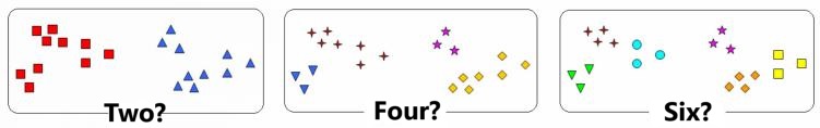
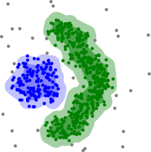
Types of Cluster Structures
Intra-cluster distances are generally smaller than inter-cluster distances
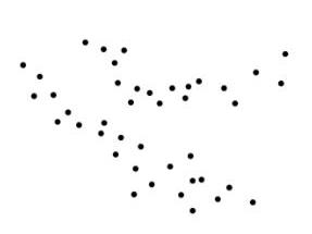
Ribbon clusters
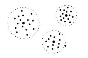
Center-based clusters
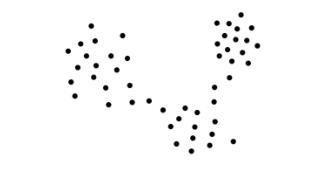
Clusters may be connected by bridges
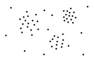
Clusters may overlay a sparse background of infrequently placed objects
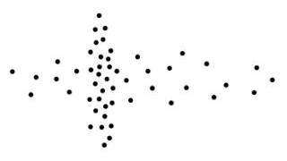
Clusters may overlap
Clusters can be formed not only by proximity but also by other types of regularities
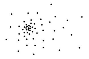
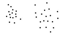
Clusters may not exist at all
- Each clustering method has its limitations and identifies only clusters of certain types
- The concept "type of cluster structure" depends on the method and also does not have a formal definition
- In the multidimensional case, all this is even more true
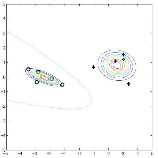
Semi-supervised Learning Task Formulation
Given: set of objects $X$, set of classes $Y$
$X^k = \begin{array}{c} \{x_1, \dots, x_k \} \\ \color{orange}{\{y_1, \dots, y_k \}} \\ \end{array}$ — labeled data$U = \{x_{k+1}, \dots, x_\ell \}$ — unlabeled data
Two variants of the task formulation:
- Semi-supervised learning (SSL): construct a classification algorithm $a: X \to Y$
- Transductive learning: knowing ${\color{orange}\text{all}}\ \{x_{k+1}, \dots, x_\ell \}$, obtain labels $\{a_{k+1}, \dots, a_\ell\}$
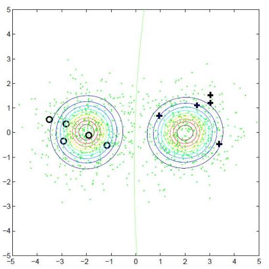
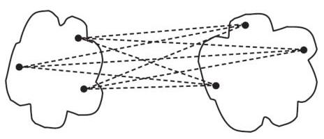
SSL Does Not Reduce to Classification
Example 1: Class densities restored.
 |
 |
| using labeled data $X^k$ | using full data $X^\ell$ |
Example 2: Classification methods do not account for the cluster structure of unlabeled data
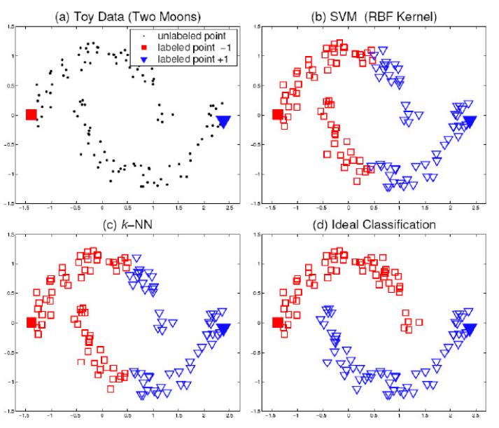
However, SSL Also Does Not Reduce to Clustering
Example 3: Clustering methods do not consider the priority of labeling over cluster structure. How to classify objects in clusters:
Clustering Quality Criteria
Suppose only pairwise distances between objects are known.
Average intra-cluster distance:
$$F_0 = \frac{\sum\limits_{i < j}[a_i = a_j] \rho(x_i, x_j)}{\sum\limits_{i < j}[a_i = a_j]} \to \min$$Average inter-cluster distance:
$$F_1 = \frac{\sum\limits_{i < j}[a_i \neq a_j] \rho(x_i, x_j)}{\sum\limits_{i < j}[a_i \neq a_j]} \to \max$$Ratio of functionals: $F_0 / F_1 \to \min$
Clustering Quality Criteria in Vector Space
Let the objects \(x_i\) be represented by vectors of features \( (f_1(x_i),\dots,f_n(x_i)) \)
-
Sum of average intra-cluster distances:
\[ \Phi_0 = \sum\limits_{a \in Y} \frac{1}{|X_a|} \sum\limits_{i: a_i = a} \rho(x_i, \mu_a) \to \min \]
\( X_a = \{x_i \in X^\ell | a_i = a\} \) — cluster \( a \), \( \mu_a \) — centroid of cluster \( a \)
-
Sum of inter-cluster distances:
\[ \Phi_1 = \sum\limits_{a, b \in Y} \rho(\mu_a, \mu_b) \to \max \]
-
Ratio of functionals: $ \Phi_0 / \Phi_1 \to \min $
Clustering as a Discrete Optimization Problem
Weights on pairs of objects (proximity): \( w_{ij} = \exp(-\beta \rho(x_i, x_j)) \), where \( \rho(x, x^\prime) \) is the distance between objects, \( \beta \) is a parameter
Clustering Task:
Find cluster labels \(a_i:\ \sum\limits_{i=1}^\ell \sum\limits_{j=i+1}^\ell w_{ij} [a_i \neq a_j] \to \min\limits_{\{a_i \in Y\}}\)
Partial Learning Task:
$$ \sum\limits_{i=1}^\ell \sum\limits_{j=i+1}^\ell w_{ij} [a_i \neq a_j] + {\color{orange}\lambda \sum\limits_{i=1}^k [a_i \neq y_i]} \to \min\limits_{\{a_i \in Y\}}$$where \(\lambda\) is another parameter
k-means Method for Clustering
Minimization of the sum of squared intra-class distances:
\[ \sum\limits_{i=1}^\ell \|x_i - \mu_{a_i} \|^2 \to \min\limits_{\{a_i\}, \{\mu_a\}},\\ \|x_i - \mu_{a} \|^2 = \sum\limits_{j=1}^n (f_j(x_i) - \mu_{a_j})^2 \]
Lloyd's Algorithm for k-means
Input: \(X^\ell, K = |Y|\)
Output: cluster centers \( \mu_a \) and labels \( a \in Y \)
- \( \mu_a = \) initial approximation of centers, for all \( a \in Y \)
- Repeat
- First step: assign each \( x_i \) to the nearest center:
\( a_i = \arg\min\limits_{a \in Y} \|x_i - \mu_a \|, i = 1, \dots, \ell \) - Second step: calculate new positions of centers:
\( \mu_{a_j} = \frac{\sum\limits_{i = 1}^\ell [a_i = a] x_i}{\sum\limits_{i = 1}^\ell [a_i = a]}, a \in Y \) - Until \( a_i \) stop changing
k-means++
- Randomly and uniformly select a center \( c_1 \) from \( X \)
- Repeat \( k - 1 \) times
$\ \ \ $ Choose \( x \in X \) as the center of a new cluster with probability \( \frac{D^2(x)}{\sum\limits_{x \in X} D^2(x)} \) - Use the standard k-means algorithm
* Here \( D(x) \) is the distance from \( x \) to the nearest cluster
David Arthur and Sergei Vassilvitskii. k-means++: The Advantages of Careful Seeding, 2007
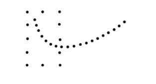
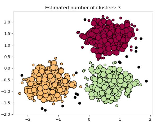
Examples of Unsuccessful k-means Clustering
Reason: unfortunate initial approximation and "ribbon-like" clusters
k-means Modification for Semi-Supervised Learning
Given labeled objects \( \{x_1, \dots, x_k\} \), with \( \color{orange}{U} \) being the set of unlabeled objects
Input: \( X^\ell, K = |Y| \). Output: cluster centers \( \mu_a, a \in Y \)
- \( \mu_a = \) initial approximation of centers, for all \( a \in Y \)
- Repeat
- First step: assign each \( x_i \in {\color{orange}U} \) to the nearest center:
\( a_i = \arg\min\limits_{a \in Y} \|x_i - \mu_a \|, i = {\color{orange}k+1, \dots, \ell}\) - Second step: calculate new positions of centers:
\( \mu_{a_j} = \frac{\sum\limits_{i = 1}^\ell [a_i = a] x_i}{\sum\limits_{i = 1}^\ell [a_i = a]}, a \in Y \) - Until \( a_i \) stop changing
Let's have a break!
DBSCAN Clustering Algorithm
DBSCAN — Density-Based Spatial Clustering of Applications with Noise
Consider an object \( x \in U \), and its \( \varepsilon \)-neighborhood \[ U_\varepsilon(x) = \{ u \in U: \rho(x,u) \leq \varepsilon\} \]
Each object can be one of three types:
- core: having a dense neighborhood, \( |U_\varepsilon (x)| \geq m \)
- border: not core, but in the neighborhood of a core
- noise (outlier): neither core nor border
Ester, Kriegel, Sander, Xu. A density-based algorithm for discovering clusters in large spatial databases with noise. KDD-1996
DBSCAN Clustering Algorithm
Input: dataset \( X^\ell = \{x_1, \dots, x_\ell\} \), parameters \( \varepsilon \) and \( m \)
Output: partition of the dataset into clusters and noise points
\( U = X^\ell \) — unlabeled, \( a = 0 \)
While there are unlabeled points in the dataset, i.e. \( U \neq \emptyset \):
- Take a random point \( x \in U \)
- If \( |U_\varepsilon (x)| < m \) then mark \( x \) as potentially noisy
- Else
- create a new cluster: \( K = U_\varepsilon(x), a = a + 1 \)
- for all \( x^\prime \in K \), not marked or noisy
- if \( |U_\varepsilon(x^\prime)| \geq m \) then \( K = K \cup U_\varepsilon(x^\prime) \)
- else mark \( x^\prime \) as a border of cluster \( K \)
- \( a_i = a \) for all \( x_i \in K \)
- \( U = U/K \)
Advantages of the DBSCAN Algorithm
- Fast clustering of large data:
- \( O(\ell^2) \) in the worst case
- \( O(\ell\ln \ell) \) with efficient implementation of \( U_\varepsilon(x) \)
- Clusters of arbitrary shapes (no centers)
- Classification of objects into core, border, and noise
Agglomerative Hierarchical Clustering
Algorithm of hierarchical clustering (Lance, Williams, 1967):
Iterative recalculation of distances \( R_{UV} \) between clusters \( U, V \)
- \( С_1 = \{\{x_1\},\dots, \{x_\ell\}\} \) — all clusters are 1-element
\( R_{\{x_i\}\{x_j\}} = \rho(x_i, x_j) \) — distances between them - for all \( t = 2, \dots, \ell \) (\( t \) — iteration number):
- Find in \( C_{t-1} \) a pair of clusters \( (U, V) \) with minimal \( R_{UV} \)
- Merge them into one cluster:
\( W = U \cup V \)
\( С_t = С_{t-1} \cup \{W\}/\{U,V\} \) - for all \( S \in C_t \) calculate \(R_{WS}\) using Lance-Williams formula:
\( R_{WS} = \alpha_U R_{US} + \alpha_V R_{VS} + \beta R_{UV} + \gamma |R_{US} - R_{VS}| \)
Specific Cases of the Lance-Williams Formula
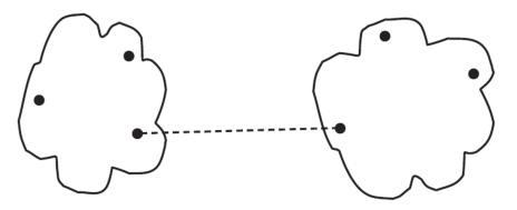
1. Nearest neighbor distance:
\( R^{\text{nn}}_{WS} = \min_{w \in W, s\in S} \rho (w,s) \)
\( \alpha_{U} = \alpha_{V} = \frac12, \beta = 0, \gamma = -\frac12 \)
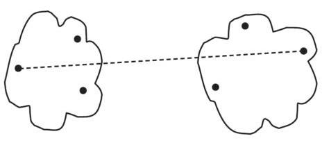
2. Farthest neighbor distance:
\( R^{\text{fn}}_{WS} = \max_{w \in W, s\in S} \rho (w,s) \)
\( \alpha_{U} = \alpha_{V} = \frac12, \beta = 0, \gamma = \frac12 \)
3. Group average distance:
\( R^{\text{g}}_{WS} = \frac{1}{|W| |S|} \sum\limits_{w \in W} \sum\limits_{s \in S} \rho(w, s) \)
\( \alpha_{U} = \frac{|U|}{|W|}, \alpha_{V} = \frac{|V|}{|W|}, \beta = \gamma = 0 \)
Specific Cases of the Lance-Williams Formula
- Distance between centroids:
\( R^{\text{c}}_{WS} = \rho^2\left(\sum\limits_{w \in W} \frac{w}{|W|}, \sum\limits_{s \in S} \frac{s}{|S|} \right) \)
\( \alpha_{U} = \frac{|U|}{|W|}, \alpha_{V} = \frac{|V|}{|W|}, \beta = -\alpha_{U}\alpha_{V}, \gamma = 0 \)
- Ward's distance:
\( R^{\text{w}}_{WS} = {\color{orange}\frac{|S||W|}{|S|+|W|}} \rho^2\left(\sum\limits_{w \in W} \frac{w}{|W|}, \sum\limits_{s \in S} \frac{s}{|S|} \right) \)
\( \alpha_{U} = \frac{|S|+|U|}{|S|+|W|}, \alpha_{V} = \frac{|S|+|V|}{|S|+|W|}, \beta = \frac{-|S|}{|S|+|W|}, \gamma = 0 \)
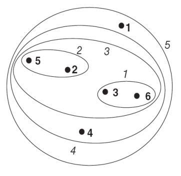
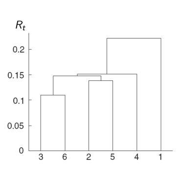
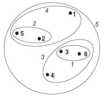
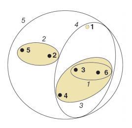
Visualization of Cluster Structure
1. Nearest Neighbor Distance
| Embedding Diagram | Dendrogram |
|---|---|
 |
 |
2. Farthest Neighbor Distance
| Embedding Diagram | Dendrogram |
|---|---|
 |
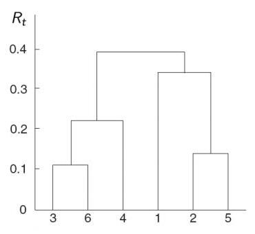 |
Main Properties of Hierarchical Clustering
- Monotonicity: the dendrogram has no self-intersections, and with each merge, the distance between the clusters being combined only increases:
\( R_2 \leq R_3 \leq \dots \leq R_\ell \) - Contraction Distance: \( R_t \leq \rho(\mu_U, \mu_V), \forall t \)
- Expansion Distance: \( R_t \geq \rho(\mu_U, \mu_V), \forall t \)
Theorem (Milligan, 1979): Clustering is monotonic if the conditions \( \alpha_U \geq 0, \alpha_V \geq 0, \alpha_U + \alpha_V + \beta \geq 1, \min\{\alpha_U, \alpha_V\} + \gamma \geq 0 \) are met
\( R^\text{c} \) is not monotonic; \( R^\text{nn} \), \( R^\text{fn} \), \( R^\text{g} \), \( \color{orange}{R^\text{w}} \) are monotonic
\( R^\text{nn} \) is contracting; \( R^\text{fn}, \color{orange}{R^\text{w}} \) are expanding
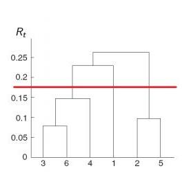
Recommendations about Hierarchical Clustering
- It is recommended to use Ward's distance \( R^\text{w} \)
- Usually, several variants are constructed and the best one is chosen visually based on the dendrogram
- The number of clusters is determined by the maximum of \( |R_{t+1} - R_t| \),
then the resulting set of clusters \( = C_t \)
 |
 |
Self-Training Method in Semi-Supervised Learning
Let \( \mu: X^k \to a \) be a method for learning classification
Classifiers are of the form \( a(x) = \arg\max\limits_{y \in Y} \Gamma_y(x) \) , where \(\Gamma_y(x)\) is raw score
Pseudo-margin — the degree of confidence in the classification \( a_i = a(x_i) \):
\[ \boxed{ M_i(a) = \Gamma_{a_i}(x_i) - \max\limits_{y \in Y/a_i} \Gamma_y(x_i)} \]Self-Training Algorithm
Self-Training Algorithm — a wrapper over the method \( \mu \):
- \( Z = X^k \)
- While \( |Z| < \ell \)
- \( a = \mu(Z) \)
- \( \Delta = \{x_i \in U/Z | M_i(a) \geq \color{orange}{M_0}\} \)
- \( a_i = a(x_i) \) for all \( x_i \in \Delta \)
- \( Z = Z \cup \Delta \)
\( \color{orange}{M_0} \) can be determined, for example, from the condition \( |\Delta| = 0.05 |U| \)
Semi-Supervised Learning Method: Co-Learning (deSa, 1993)
Let \( \mu_t: X^k \to a_t \) be different learning methods, \( t = 1, \dots, T \)
Co-learning Algorithm is self-training for a composition — simple voting of base algorithms \( a_1, \dots, a_T \):
\[ \boxed{a(x) = \arg\max\limits_{y in Y} \Gamma_y(x),\ \Gamma_y(x_i) = \sum\limits_{t=1}^T[a_t(x_i) = y]} \]Semi-Supervised Learning Method: Co-Training (Blum, Mitchell, 1998)
Let \( \mu_1: X^k \to a_1,\ \mu_2: X^k \to a_2 \) be two substantially different learning methods, using either:
- different sets of features
- different learning paradigms (inductive bias)
- different data sources \( X_1^{k_1}, X_2^{k_2} \)
- \( Z_1 = X_1^{k_1} \), \( Z_2 = X_2^{k_2} \)
- While \( |Z_1 \cup Z_2| < \ell \)
- \( a_1 = \mu_1(Z_1), \Delta_1 = \{x_i \in U/Z_1/Z_2 | M_i(a_1) \geq {\color{orange}M_{01}}\} \)
- \( a_i = a_1(x_i) \) for all \( x_i \in \Delta_1 \)
- \( Z_2 = Z_2 \cup \Delta_1 \)
- \( a_2 = \mu_2(Z_2), \Delta_2 = \{x_i \in U/Z_1/Z_2 | M_i(a_2) \geq {\color{orange}M_{02}}\} \)
- \( a_i = a_2(x_i) \) for all \( x_i \in \Delta_2 \)
- \( Z_1 = Z_1 \cup \Delta_2 \)
Summary
- Clustering is unsupervised learning, an ill-posed problem; there exist many optimization and heuristic algorithms for clustering
- DBSCAN is a classic and fast clustering algorithm
- The task of semi-supervised learning (SSL) occupies an intermediate position between classification and clustering but does not reduce to one of them
- Clustering methods are easily adapted to SSL by introducing constraints (constrained clustering)
- Adapting classification methods is more complex, involving additional regularization, and typically leads to more effective methods
- Regularization combines criteria on labeled and unlabeled data into a single optimization task
What else to look at?
Lance-Williams Algorithm for Semi-Supervised Learning (1967)
- \( С_1 = \{\{x_1\},\dots, \{x_\ell\}\} \) — all clusters are 1-element
\( R_{\{x_i\}\{x_j\}} = \rho(x_i, x_j) \) — distances between them - for all \( t = 2, \dots, \ell \) (\( t \) — iteration number):
- Find in \( C_{t-1} \) a pair of clusters \( (U, V) \) with minimal \( R_{UV} \)
under the condition that \( U \cup V \) does not contain objects with different labels - Merge them into one cluster:
\( W = U \cup V \), \( С_t = С_{t-1} \cup \{W\}/\{U,V\} \) - for all \( S \in C_t \) calculate \( R_{WS} \) using the Lance-Williams formula:
\( R_{WS} = \alpha_U R_{US} + \alpha_V R_{VS} + \beta R_{UV} + \gamma |R_{US} - R_{VS}| \)