Advanced machine learning
Expectation-Minimization algorithm
Alex Avdiushenko
February 11, 2025

KL divergence
Let's start with a well-known fact
Jensen's Inequality
If \( f(x) \) is a concave (upward-convex) function, then Jensen's inequality holds:
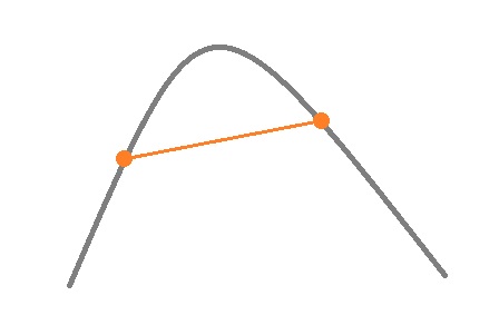
Or, in a more general case,
\[f(w_1x_1 + w_2x_2 + \dots + w_nx_n) \geq w_1f(x_1) + w_2f(x_2) + \dots + w_nf(x_n)\]where \( \sum\limits_{i=1}^n w_i = 1 \).
It can also be proven that
\[ f\left(\mathbb{E}_{p(x)} u(x)\right) \geq \mathbb{E}_{p(x)} f(u(x)) \]Kullback-Leibler Divergence Between Probability Distributions
\[ KL(p||q) = \int p(x) \log \frac{p(x)}{q(x)} dx \] represents how much information is "lost" when $q$ is used to approximate $p$
Properties:
- \( KL(p||q) \neq KL(q||p) \) — asymmetry
- \( KL(p||q) \geq 0 \) — non-negativity
- \( KL(p||q) = 0 \Leftrightarrow q(x) = p(x) \)
Proof of non-negativity of KL divergence:
\[ -KL(p||q) = -\int p(x) \log\left(\frac{p(x)}{q(x)}\right)dx = \int p(x) \log\left(\frac{q(x)}{p(x)}\right)dx \leq \\ \leq \log\left( \int p(x) \frac{q(x)}{p(x)}dx\right) = \log\left( \int q(x) dx\right) = \log 1 = 0 \]Connecting KL Divergence and Cross-Entropy
Recall the entropy of $p$: \[ H(p) = -\int p(x) \log p(x) dx \]
Cross-Entropy: \[ H(p, q) = -\int p(x) \log q(x) dx \]
KL Divergence: \[ KL(p||q) = -H(p) + H(p,q) \]
Asymmetry of KL Divergence
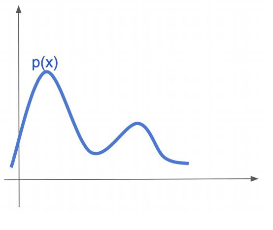
Example: searching for a similar distribution
\( KL(? || ?) \) — where to place \( p \)?
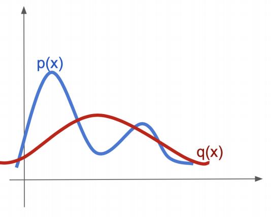
First argument: mass covering
\[ KL(p || q) = \int p(x) \log \frac{p(x)}{q(x)} dx \]
Second argument: mode collapsing
\[ KL(q || p) = \int q(x) \log \frac{q(x)}{p(x)} dx \]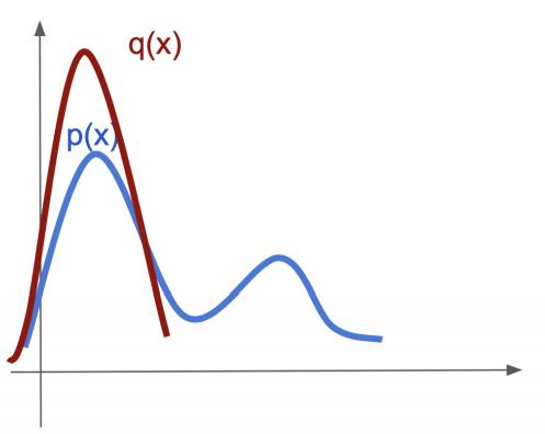

EM-Algorithm: Motivating Example
How can we learn to reconstruct distributions?
Gaussian:
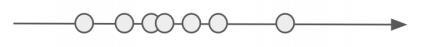
Multiple Gaussians:

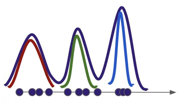
Unknown Distribution:
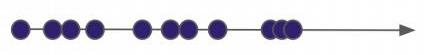
We can introduce the Gaussian number and reduce the problem to an already solved one (as in joke with electric kettle, yeah)!
Introducing Latent Variables
We want: $$p(X|\theta) \underset{\theta}{\to} \max \text{(incomplete likelihood)}$$
We can: $$p(X, Z|\theta) \underset{\theta}{\to} \max \text{(complete likelihood)}$$
Let's say in the previous example, $z_i$ is the identifier of the Gaussian from which the $i$-th object is taken
Variational Lower Bound
For a single observation $x$:
$$ \begin{align*} \log p(x|\theta) &= \int q(z) \log p(x|\theta) dz = \int q(z) \log \frac{p(x, z|\theta)}{p(z|x,\theta)} dz \\ &= \int q(z) \log \frac{p(x, z|\theta)q(z)}{p(z|x,\theta)q(z)} dz\\ &= \int q(z) \log \frac{p(x, z|\theta)}{q(z)} dz + \int q(z) \log \frac{q(z)}{p(z|x,\theta)} dz \geq\\ &\geq \int q(z) \log \frac{p(x, z|\theta)}{q(z)} dz = \mathscr{L}(q, \theta) \end{align*} $$This is the variational lower bound: we simply discarded the non-negative $KL(q(z) || p(z|x,\theta))$. Furthermore, equality is reached at $q^* = p(z| x, \theta)$
For dataset $X$:
$$ \log p(X| \theta) = \sum\limits_{i=1}^n \log p(x_i|\theta) \geq \sum\limits_{i=1}^n \mathscr{L}(q_i, \theta) \underset{q, \theta}{\to} \max $$It's easy to maximize for $\theta$ if we know $q$ and vice versa.
EM-Algorithm
E-step (Expectation):
$$ \sum\limits_{i=1}^n \mathscr{L}(q_i, \theta) \underset{q_i}{\to} \max \Leftrightarrow q_i(z_i) = p(z_i|x_i, \theta) $$M-step (Maximization):
$$ \begin{align*} \max\limits_\theta \sum\limits_{i=1}^n \mathscr{L}(q_i, \theta) &= \max\limits_\theta \sum\limits_{i=1}^n \int q_i(z_i) \log\frac{p(x_i, z_i| \theta)}{q_i(z_i)} dz_i \\ &= \max\limits_\theta \sum\limits_{i=1}^n E_{q_i(z_i)} \log p(x_i, z_i| \theta) \end{align*} $$
Gaussian Mixture Model
The joint probability of $x_i$ and $z_i$ given $\theta$ can be represented as:
$$ p(x_i, z_i|\theta) = p(x_i|z_i,\theta)p(z_i|\theta) = N(x_i|\mu_{z_i}, \sigma_{z_i}^2) \pi_{z_i} $$Parameters: $\{\mu_j, \sigma_j, \pi_j\}$, where $\pi_j$ is a priori probability of the $j$-th Gaussian (hidden variable $z_i$)
- We can use simple enumeration based on their quantity (model selection method)
- We can take a different approach — introduce a prior distribution directly on all models of different complexity. This is the main idea of Bayesian nonparametric methods
- Also see the "Chinese Restaurant Process" and "Indian Buffet Process" for solution
EM-Algorithm for Gaussian Mixture Model
E-step: $\mu_k, \sigma_k^2, \pi_k \to q$
$$ q_i(z_i{\scriptsize =}j) = p(z_i{\scriptsize =}j|x_i, \theta) = \frac{p(x_i|z_i {\scriptsize =} j, \theta)p(z_i {\scriptsize =} j|\theta)}{p(x_i|\theta)} = \\ \frac{p(x_i|z_i {\scriptsize =} j, \theta)p(z_i {\scriptsize =} j|\theta)}{\sum\limits_{k=1}^K p(x_i|z_i {\scriptsize =} k, \theta)p(z_i {\scriptsize =} k|\theta)} = \frac{N(x_i|\mu_j, \sigma_j^2) \pi_j}{\sum\limits_{k=1}^K N(x_i|\mu_k, \sigma_k^2) \pi_k} $$M-step: $q \to \mu_k, \sigma_k^2, \pi_k$
$$ \begin{align*} \sum\limits_{i=1}^n \mathscr{L}(q,\theta) & = \sum\limits_{i=1}^n \sum\limits_{k=1}^K q_i(z_i{\scriptsize =}k) \log\frac{p(x_i|z_i {\scriptsize =} k, \theta)p(z_i {\scriptsize =} k|\theta)}{q_i(z_i{\scriptsize =}k)} \\ & = \sum\limits_{i=1}^n \sum\limits_{k=1}^K q_i(z_i{\scriptsize =}k) \log\frac{N(x_i|\mu_k, \sigma_k^2)\pi_k}{q_i(z_i{\scriptsize =}k)} \end{align*} $$Next, as usual, we find the zeros of the derivative:
$$ \mu_j = \frac{\sum\limits_{i=1}^n q_i(z_i{\scriptsize =}j)x_i}{\sum\limits_{i=1}^n q_i(z_i{\scriptsize =}j)}; \; \sigma_j^2 = \frac{\sum\limits_{i=1}^n q_i(z_i{\scriptsize =}j)(x_i-\mu_j)^2}{\sum\limits_{i=1}^n q_i(z_i{\scriptsize =}j)} \\ \pi_j = \frac{1}{n} \sum\limits_{i=1}^n q_i(z_i {\scriptsize =} j) $$Let's have a break!
Principal Component Analysis: Problem Formulation
$f_1(x), \dots, f_D(x)$ — original numerical features
$g_1(x), \dots, g_d(x)$ — new numerical features, $d \leq D$
Requirement: The old features should be restored as accurately as possible linearly from the new ones on the training set $X^n$:
$$ \hat f_j(x) = \sum\limits_{s=1}^d g_s(x) u_{js}, j=1,\dots,D , \forall x \in X $$ $$ \sum\limits_{i=1}^n \sum\limits_{j=1}^D (\hat f_j(x_i) - f_j(x_i))^2 \to \min\limits_{\{g_s(x_i)\}, \{u_{js}\}} $$Matrix Notations
Old and new "object-feature" matrices:
$$ F_{n \times D} = \left[ \begin{array}{ccc} f_1(x_1) & \dots & f_D(x_1) \\ \dots & \dots & \dots \\ f_1(x_n) & \dots & f_D(x_n) \end{array} \right] \ ,\\[.5cm] G_{n \times d} = \left[ \begin{array}{ccc} g_1(x_1) & \dots & g_d(x_1) \\ \dots & \dots & \dots \\ g_1(x_n) & \dots & g_d(x_n) \end{array} \right] $$The transformation of old features into new ones should be linear:
$$ U_{D \times d} = \left[ \begin{array}{ccc} u_{11} & \dots & u_{1d} \\ \dots & \dots & \dots \\ u_{D1} & \dots & u_{Dd} \end{array} \right], \hat F = GU^T \underset{\text{desired}}{\approx} F $$To find: both new features $G$, and transformation $U$:
$$ \sum\limits_{i=1}^n \sum\limits_{j=1}^D (\hat f_j(x_i) - f_j(x_i))^2 = \| GU^T - F\|^2 \to \min\limits_{G,U} $$Probabilistic Interpretation of the Principal Component Analysis (PPCA)
$$ p(x,z|\theta) = p(x|z, \theta)p(z) = N(x|Wz + \mu, \sigma^2I)N(z|0, I), $$where $x \in R^D$, $z \in R^d$ and $z \sim N(0, I)$
The parameters are ${W, \mu, \sigma}$, where $\mu \in R^D$, $W \in R^{D\times d}$
EM-Algorithm for Probabilistic Principal Component Analysis
E-step (is calculated analytically, as conjugate distributions exist):
$$ q_i(z_i) = p(z_i|x_i, \theta) = \frac{p(x_i|z_i, \theta)p(z_i)}{\int p(x_i|z_i, \theta)p(z_i) dz_i} = \\[.2cm] = N(z_i| (\sigma^2I + W^TW)^{-1}W^T (x_i - \mu), (I + \sigma^{-2}W^TW)^{-1}) $$M-step:
$$ E_Z\log p(X, Z|\theta) = \sum\limits_{i=1}^n E_{z_i} \log p(x_i, z_i|\theta) = \\ \sum\limits_{i=1}^n E_{z_i} \log p(x_i| z_i, \theta) + const \underset{\theta}{\to} \max $$M-step example: finding W
$$ \sum\limits_{i=1}^n E_{z_i} \log p(x_i| z_i, \theta) = \\ = \sum\limits_{i=1}^n E_{z_i} \left[-\frac{D}{2}\log2\pi-D\log\sigma-\frac{1}{2\sigma^2}\left((x_i - \mu)-Wz_i\right)^T\left((x_i - \mu)-Wz_i\right) \right] = \\ = const(\sigma) - \frac{1}{2\sigma^2} \sum\limits_{i=1}^n E_{z_i} \left[(x_i - \mu)^T(x_i - \mu) - 2(x_i - \mu)^T Wz_i + z_i^TW^T Wz_i \right] = \\ = const(\sigma) - \\ - \frac{1}{2\sigma^2} \sum\limits_{i=1}^n \left[(x_i - \mu)^T(x_i - \mu) - 2(x_i - \mu)^T W E_{z_i}z_i + tr(W^T WE_{z_i}z_iz_i^T) \right] $$Next, differentiate with respect to $W$:
$$ - \frac{1}{2\sigma^2} \sum\limits_{i=1}^n \left[-2(x_i - \mu) E_{z_i} z_i^T + 2W E_{z_i} z_i z_i^T \right] = 0 \\ W^* = \left( \sum\limits_{i=1}^n (x_i - \mu) E_{z_i} z_i^T \right) \left( \sum\limits_{i=1}^n E_{z_i} z_i z_i^T \right)^{-1} $$We can calculate the expectations since we know the distribution $q$ from the previous E-step.
Comparison of Runtime Estimates
When $n > D > d$:
- Standard PCA: $O(nD^2)$
- A single iteration of PPCA: $O(nDd)$
Usually, 10-100 iterations are needed for convergence, so it may be faster than the standard method
The case of missing features in Probabilistic Principal Component Analysis
$$ (X, Z) = X_{\text{obs}} \cup X_{\text{hid}}, P(X_{\text{obs}}|\theta) \underset{\theta}{\to} \max $$E-step
$$ q(X_{\text{hid}}) = p(X_{\text{hid}}|X_{\text{obs}}, \theta) $$M-step
$$ E_{X_\text{hid}} \log p(X_{\text{obs}}, X_{\text{hid}} |\theta) \underset{\theta}{\to} \max $$And we also obtain suitable probabilistic distributions for hidden variables
Summary
- A common "metric" between probabilistic distributions is the Kullback-Leibler distance (KL-divergence)
- The EM algorithm allows iterative solutions to complex problems by dividing them into two steps
- Probabilistic Principal Component Analysis used the EM algorithm